Detecting synchronization in spatially extended discrete systems by complexity measurements

Abstract

The synchronization of two stochastically coupled one-dimensional cellular automata (CA) is analyzed. It is shown that the transition to synchronization is characterized by a dramatic increase of the statistical complexity of the patterns generated by the difference automaton. This singular behavior is verified to be present in several CA rules displaying complex behavior.

Despite all the efforts devoted to understand the meaning of complexity, we still do not have an instrument in the laboratories specially designed for quantifying this property. Maybe this is not the final objective of all those theoretical attempts carried out in the most diverse fields of knowledge in the last years grassberger ; lloyd ; shiner ; kolmogorov ; chaitin ; lempel ; bennett ; crutchfield , but, for a moment, let us think in that possibility.

Similarly to any other device, our hypothetical apparatus will have an input and an output. The input could be the time evolution of some variables of the system. The instrument records those signals, analyzes them with a proper program and finally screens the result in the form of a complexity measurement. This process is repeated for several values of the parameters controlling the dynamics of the system. If our interest is focused in the more complex configuration of the system we have now the possibility of tuning such an state by regarding the complexity plot obtained at the end of this process.

As a real applicability of this proposal, let us apply it to an à-la-mode problem. The clusterization or synchronization of chaotic coupled elements was put in evidence at the beginning of the nineties kaneko ; lopez91 . Since then, a lot of publications have been devoted to this subject boccaletti . Let us consider one particular of these systems to illuminate our proposal.

(1) SYSTEM: We take two coupled elementary one dimensional cellular automata displaying complex spatio-temporal dynamics wolfram . Recently, it has been show that this system can undergo through a synchronization transition zanette . The transition to full synchronization occurs at a critical value $p_{c}$ of a synchronization parameter $p$. Briefly the numerical experiment is as follows. Two $L$-cell cellular automata (CA) with the same evolution rule $\Phi$ are started from different random initial conditions for each automaton. Then, at each time step, the dynamics of the coupled CA is governed by the successive application of two evolution operators; the independent evolution of each CA according to its corresponding rule $\Phi$ and the application of a stochastic operator that compares the states $\sigma_{i}^{1}$ and $\sigma_{i}^{2}$ of all the cells, $i=1,...L$, in each automaton. If $\sigma_{i}^{1}=\sigma_{i}^{2}$, both states are kept invariant. If $\sigma_{i}^{1}\neq\sigma_{i}^{2}$, they are left unchanged with probability $1-p$, but both states are updated either to $\sigma_{i}^{1}$ or to $\sigma_{i}^{2}$ with equal probability $p/2$. It is shown in reference zanette that there exists a critical value of the synchronization parameter ($p_{c}=0.193$ for the rule $18$) above which full synchronization is achieved.

(2) DEVICE: We choose a particular instrument to perform our measurements, that capable of displaying the value of the LMC complexity ($C$) LMC . The statistical complexity $C$ is defined as follows,

$$C(\{\rho_{i}\}) = H(\{\rho_{i}\})\cdot D(\{\rho_{i}\})\;=$$ (1)

$$= -k\left[\sum_{i=1}^{N}\rho_{i}\log\rho_{i}\right]\times\>\left[\sum_{i=1}^{N}\,\left(\rho_{i}-\frac{1}{N}\right)^{2}\right]\>,$$

where $\{\rho_{i}\}$ represents the set of probabilities of the $N$ accessible discrete states of the system, with $\rho_{i}\geq 0$ , $i=1,\cdots,N$, and $k$ is a constant. If $k=1/logN$ then we have the normalized complexity. $C$ is a statistical measure of complexity that identifies the entropy or information stored in a system and its disequilibrium, i.e., the distance from its actual state to the probability distribution of equilibrium, as the two basic ingredients for calculating the complexity of a system. This quantity vanishes both for completely ordered and for completely random systems giving then the correct asymptotic properties required for a such well-behaved measure. The calculation of $C$ has been useful to successfully discern many situations regarded as complex in discrete systems out of equilibrium calbet ; martin ; guozhang ; zuguo ; lovallo .

(3) INPUT: In particular the evolution of two coupled CA evolving under the rules $22$, $30$, $90$ and $110$ is analyzed. The pattern of the difference automaton will be the input of our device. In Fig. 1 it is shown it for a coupling probability $p=0.23$, just above the synchronization transition. The left and the right plots show $250$ successive states of the two automata, whereas the central plot displays the corresponding difference automaton. Such automaton is constructed by comparing one by one all the sites ($L=100$) of both automata and putting zero when the states $\sigma_{i}^{1}$ and $\sigma_{i}^{2}$, $i=1\ldots L$, are equal or putting one otherwise. It is worth to observe that the difference automaton shows an interesting complex structure close to the synchronization transition. This complex pattern is only found in this region of parameter space. When the system if fully synchronized the difference automaton is composed by zeros in all the sites, while when there is no synchronization at all the structure of the difference automaton is completely random.

(4) METHOD OF MEASUREMENT: How to perform the measurement of $C$ for such two-dimensional patterns has been presented recently in Ref. LR-S . We let the system evolve until the asymptotic regime is attained. The variable $\sigma_{i}^{d}$ in each cell of the difference pattern is successively translated to an unique binary sequence when the variable $i$ covers the spatial dimension of the lattice, $i=1,\ldots,L$, and the time variable $n$ is consecutively increased. This binary string is analyzed in blocks of $n_{o}$ bits, where $n_{o}$ can be considered the scale of observation. The accessible states to the system among the $2^{n_{o}}$ possible states is found as well as their probabilities. Then, the magnitudes $H$, $D$ and $C$ are directly calculated and screened by the device.

(5) OUTPUT: The results of the measurement are shown in Fig. 2. The normalized complexity $C$ as a function of the synchronization parameter $p$ is plotted for different coupled one-dimensional CA that evolve under the rules $22$, $30$, $90$ and $110$ , which are known to generate complex patterns. All the plots of Fig. 2 were obtained using the following parameters: number of cell of the automata, $L=1000$; total evolution time, $T=600$ steps. For all the cases and scales analyzed, the statistical complexity $C$ shows a dramatic increase close to the synchronization transition. It reflects the complex structure of the difference automaton and the capability of the measurement device here proposed for clearly signaling the synchronization transition of two coupled CA.

These results are in agreement with the measurements of $C$ performed in the patterns generated by a one-dimensional logistic coupled map lattice in Ref. LR-S . There the LMC statistical complexity ($C$) also shows a singular behavior close to the two edges of an absorbent region where the lattice displays spatio-temporal intermittency. Hence, in our present case, the synchronization region of the coupled systems can be interpreted as an absorbent region of the difference system. In fact, the highest complexity is reached on the border of this region for $p\approx 0.2$. The parallelism between both systems is therefore complete.

Finally, let us remark that the critical parameter for switching synchronization in these systems is similar for all of them ($p_{c}\approx 0.2$). This fact could deserve some operational explanation in a future work.

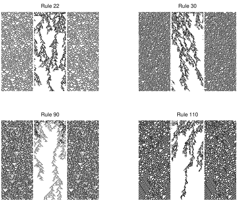
Figure 1: Spatio-temporal patterns just above the synchronization transition. The left and the right plots show $250$ successive states of the two coupled automata and the central plot is the corresponding difference automaton for the rules $22$, $30$, $90$ and $110$. The number of sites is $L=100$ and the coupling probability is $p=0.23$.

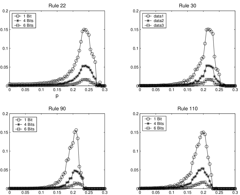
Figure 2: The normalized complexity $C$ versus the coupling probability $p$ for different scales of observation: $n_{o}=1$ ($\circ$),$n_{o}=4$ ($\star$) and $n_{o}=6$ ($\Box$). $C$ has been calculated over the last $300$ iterations of a running of $600$ of them for a lattice with $L=1000$ sites. The synchronization transition is clearly depicted around $p\approx 0.2$ for the different rules.

References

- (1) P. Grassberger, Int. J. Theor. Phys. 25, 907 (1986).
- (2) S. Lloyd and H. Pagels, Ann. Phys. (NY) 188, 186 (1988).
- (3) J.S. Shiner, M. Davison and P.T. Landsberg, Phys. Rev. E 59, 1459 (1999).
- (4) A.N. Kolmogorov, Probl. Inform. Theory 1, 3 (1965).
- (5) G. Chaitin, J. Assoc. Comput. Mach. 13, 547 (1966).
- (6) A. Lempel and J. Ziv, IEEE Trans. Inform. Theory 22, 75 (1976).
- (7) C.H. Bennett, in Emerging syntheses in science, Ed. D. Pines, Addisson-Wesley, Reading MA (1988).
- (8) J.P. Crutchfield and K. Young, Phys. Rev. Lett. 63, 105 (1989).
- (9) K. Kaneko, Phys. Rev. Lett. 63, 219 (1989); Physica D 41, 137 (1990).
- (10) R. López-Ruiz and C. Pérez-Garcia, Chaos, Solitons and Fractals 1, 511 (1991).
- (11) S. Boccaletti, J. Kurths, G. Osipov, D.L. Valladares and C.S. Zhou, Phys. Rep. 366, 1 (2002).
- (12) S. Wolfram, Rev. Mod. Phys. 55, 601 (1983).
- (13) L. G. Morelli and D. H. Zanette, Phys. Rev. E 58, R8 (1998).
- (14) R. López-Ruiz, H.L. Mancini and X. Calbet, Phys. Lett. A 209, 321 (1995).
- (15) X. Calbet and R. López-Ruiz, Phys. Rev. E 6, 066116(9) (2001).
- (16) M.T. Martin, A. Plastino and O.A. Rosso, Phys. Lett. A 311 (2-3), 126 (2003).
- (17) G. Feng and S. Song and P. Li, J. Hydr. Eng. Chin. (Hydr. Eng. Soc.) 11, article no. 14 (1998).
- (18) Z. Yu and G. Chen, Comm. Theor. Phys. (Beijing China) 33 673 (2000).
- (19) M. Lovallo, V. Lapenna and L. Telesca, Chaos, Solitons and Fractals 24, 33 (2005).
- (20) J. R. Sánchez and R. López-Ruiz. nlin.PS/0410062, submitted for publication (2004).