Finite-gap Solutions of the Vortex Filament Equation, I

Abstract.

For the class of quasi-periodic solutions of the vortex filament equation we study connections between the algebro-geometric data used for their explicit construction, and the geometry of the evolving curves. We give a complete description of genus one solutions, including geometrically interesting special cases such as Euler elastica, constant torsion curves, and self-intersecting filaments. We also prove generalizations of these connections to higher genus.

1. Introduction

In 1972, H. Hasimoto [17] introduced the complex function

$$q=\tfrac{1}{2}\,\kappa\exp\left({\mathrm{i}\int\tau\,\mathrm{d}s}\right)$$ (1)

of the curvature $\kappa$ and the torsion $\tau$ of a space curve, and showed that if the position vector ${\boldsymbol{\gamma}}$ of the curve evolves according to the vortex filament equation (VFE),

$$\frac{\partial{\boldsymbol{\gamma}}}{\partial t}=\frac{\partial{\boldsymbol{\gamma}}}{\partial s}\times\frac{\partial^{2}{\boldsymbol{\gamma}}}{\partial s^{2}},$$ (2)

then the potential $q(s,t)$ is a solution of the focussing cubic nonlinear Schrödinger equation (NLS)

$$\mathrm{i}q_{t}+q_{ss}+2|q|^{2}q=0.$$ (3)

In these equations, $s$ is the arclength parameter of the curve and the spatial variable for the NLS potential, and $t$ is time. In fact, the evolving curve defines $q(s,t)$ uniquely, up to multiplication by a unit modulus constant.

The association ${\boldsymbol{\gamma}}(s,t)\mapsto q(s,t)$ is often referred to as the Hasimoto map. Since the NLS had been shown to be completely integrable by Zakharov and Shabat [35, 13], Hasimoto’s discovery meant that the VFE is also completely integrable, and possessed all the attendant structure: infinite sequences of commuting flows and common conservation laws, solution by inverse scattering, and special solutions such as solitons and, more generally, finite-gap solutions.

The VFE was proposed a century ago as a simplified model for the self-induced motion of vortex lines in an incompressible fluid [31, 25]. Hasimoto’s discovery has developed into one of the richest examples of the connection between curve geometry and integrability. The understanding of this connection has progressed in recent years along different directions. In the case of the VFE, its bihamiltonian structure and recursion operator have been given a geometrical realization [26, 32] and its relation to the NLS has been shown to possess a natural geometric interpretation [33, 5]. The study of special solutions, including solitons, finite-gap solutions and their homoclinic orbits has been undertaken by several researchers, employing techniques ranging from perturbation theory [21, 10] to methods of algebraic-geometry and Bäcklund transformations [34, 11, 7], in particular with the aim of understanding whether the presence of infinitely many symmetries and integral invariants implies restrictions on the topology of the evolving curves [28, 3].

In this paper, we focus on connections between geometric information about the evolving curve ${\boldsymbol{\gamma}}$, and features of the NLS potential $q(s,t)$. Specifically, we limit ourselves to the class VFE solutions that correspond to periodic and quasiperiodic finite-gap solutions of NLS, which (as explained in §2) may be constructed using algebro-geometric data, and it is this data which we seek to connect with the geometry (and topology) of ${\boldsymbol{\gamma}}$. Note that this choice is particularly significant for closed curves, since the finite-gap solutions are dense in the space of all periodic solutions [14], and it is therefore important to study their geometrical and topological properties.

Of course, the class of curves that correspond to finite-gap solutions of the NLS only makes sense if the Hasimoto map is invertible. In fact, the inverse map is defined using the solutions of the AKNS system for (3). As is well-known, the AKNS system consists of a pair of first-order linear systems

$$\begin{aligned} \boldsymbol{\psi}_{s}&=U\boldsymbol{\psi}\\ \boldsymbol{\psi}_{t}&=V\boldsymbol{\psi},\end{aligned}\qquad\boldsymbol{\psi}(s,t)\in{\mathbb{C}}^{2}$$ (4)

for a vector-valued function $\boldsymbol{\psi}$, for which the solvability or “zero curvature condition” $\boldsymbol{\psi}_{st}=\boldsymbol{\psi}_{ts}$ is equivalent to (3). Expressed in terms of the Pauli matrix $\sigma_{3}=\begin{pmatrix}1&0\\ 0&-1\end{pmatrix}$, the matrices on the right-hand sides in (4) are

$$U=-\mathrm{i}\lambda\sigma_{3}+\begin{pmatrix}0&\mathrm{i}q\\ \mathrm{i}\bar{q}&0\end{pmatrix},\qquad V=\mathrm{i}(|q|^{2}-2\lambda^{2})\sigma_{3}+\begin{pmatrix}0&2\mathrm{i}\lambda q-q_{s}\\ 2\mathrm{i}\lambda\bar{q}+\bar{q}_{s}&0\end{pmatrix}.$$

These matrices depend on $s$ and $t$ through the complex-valued function $q$, and on the spectral parameter $\lambda$. (In equations (1),(3) and (4), and elsewhere in this paper, our conventions have been chosen so as to be consistent with the important monograph by Belokolos, Bobenko et al. [1].) Because the first equation of (4) can be written as $L\boldsymbol{\psi}=\lambda\boldsymbol{\psi}$ for a first-order matrix differential operator $L$, $\boldsymbol{\psi}$ is known as an eigenfunction associated with $q$.

If one can compute a common solution of (4) for a given potential $q(s,t)$, then the curve that corresponds to $q$ under the Hasimoto map is obtained by means of the following reconstruction procedure:

Proposition 1.1 (after A. Sym [33], K. Pohlmeyer [29]).

Let $q(s,t)$ satisfy (3), let $\Psi(s,t;\lambda)$ be a matrix whose columns are linearly independent solutions of (4), such that $\Psi(0,0;\lambda)$ is a fixed matrix in $SU(2)$, and let

$$\Gamma(s,t)=\left.\Psi^{-1}\frac{\mathrm{d}\Psi}{\mathrm{d}\lambda}\right|_{\lambda=0}.$$ (5)

Then $\Gamma$ satisfies (2), and the curvature and torsion of $\Gamma$ satisfy (1), assuming we identify $\mathfrak{su}(2)$ with ${\mathbb{R}}^{3}$ via a linear isomorphism $F$, specified by

$$F:\begin{pmatrix}-\mathrm{i}&0\\ 0&\mathrm{i}\end{pmatrix}\mapsto\mathbf{e}_{1},\qquad F:\begin{pmatrix}0&1\\ -1&0\end{pmatrix}\mapsto\mathbf{e}_{2},\qquad F:\begin{pmatrix}0&\mathrm{i}\\ \mathrm{i}&0\end{pmatrix}\mapsto\mathbf{e}_{3}.$$

(Of course, the reason this construction makes sense is that $U,V$ take value in $\mathfrak{su}(2)$ when $\lambda\in{\mathbb{R}}$.) Thus, if we begin with a solution of (2), construct the potential $q(s,t)$, and solve the linear system, then the curve given by (5) will differ from what we started with by an isometry of ${\mathbb{R}}^{3}$.

Formula (5) has become known as the Sym-Pohlmeyer reconstruction formula. More generally, if in (5) we evaluate at an arbitrary real value of $\lambda$, i.e.,

$$\Gamma=\left.\Psi^{-1}\frac{\mathrm{d}\Psi}{\mathrm{d}\lambda}\right|_{\lambda=\Lambda_{0}},\qquad\Lambda_{0}\in{\mathbb{R}},$$ (6)

then $\Gamma$ still satisfies (2), but with a potential that differs from what we started with by the transformation $q(s,t)\mapsto\mathrm{e}^{\mathrm{i}(as-a^{2}t)}q(s-2at,t)$, $a\in{\mathbb{R}}$, which preserves solutions of (3). We will have recourse to the generalized Sym-Pohlmeyer formula (6) in order to associate a closed curve to a periodic NLS potential.

By differentiating (6) with respect to $s$, we see that the unit tangent vector $\mathbf{T}$ along ${\boldsymbol{\gamma}}$ and a pair of unit normal vectors $U_{1},U_{2}$ are given by

$$\mathbf{T}=\Psi^{-1}\begin{pmatrix}-\mathrm{i}&0\\ 0&\mathrm{i}\end{pmatrix}\Psi,\qquad\mathbf{U}_{1}=\Psi^{-1}\begin{pmatrix}0&1\\ -1&0\end{pmatrix}\Psi,\qquad\mathbf{U}_{2}=\Psi^{-1}\begin{pmatrix}0&\mathrm{i}\\ \mathrm{i}&0\end{pmatrix},$$

with the aforementioned identification of $\mathfrak{su}(2)$ and ${\mathbb{R}}^{3}$ understood. These vectors do not constitute a Frenet frame for ${\boldsymbol{\gamma}}$, but rather satisfy the generalized natural frame equations:

$$\dfrac{\mathrm{d}}{\mathrm{d}s}\begin{bmatrix}\mathbf{T}\\ \mathbf{U}_{1}\\ \mathbf{U}_{2}\end{bmatrix}=\begin{bmatrix}0&k_{1}&k_{2}\\ -k_{1}&0&\Lambda_{0}\\ -k_{2}&-\Lambda_{0}&0\end{bmatrix}\begin{bmatrix}\mathbf{T}\\ \mathbf{U}_{1}\\ \mathbf{U}_{2}\end{bmatrix},$$

where $k_{1},k_{2}$ are the natural curvatures, which in this case coincide with the real and imaginary parts of $2q$, respectively. (If $\Lambda_{0}=0$, then $(\mathbf{T},\mathbf{U}_{1},\mathbf{U}_{2})$ comprise a natural or relatively parallel adapted frame [2] along ${\boldsymbol{\gamma}}$.) The interpretation of the Hasimoto map in terms of natural curvatures, and the connection between the eigenfunction matrix $\Psi$ and the natural frame, will be used when we discuss closure conditions in §2.3.

Organization of the paper

In §2 we introduce the notion of finite-gap solutions, and give formulas for the eigenfunctions, potential and curve in terms of the algebro-geometric data—specifically a hyperelliptic Riemann surface $\Sigma$ and a positive divisor $\mathcal{D}$ on it, satisfying certain reality and genericity conditions. We also use these formulas to give conditions under which the curve is smoothly closed, and conditions under which it periodically intersects itself. (The closure conditions duplicate results of Grinevich and Schmidt [16], but here we derive them directly from the curve formulas.)

In §3 the ideas of the previous section are worked out in detail for the genus one case. In particular, we show that the resulting curves are centerlines for Kirchhoff elastic rods. We study the geometric features of curves associated with special configurations of the algebro-geometric data: we show that the elastic rod centerline becomes an Eulerian elastic curve precisely when the zeros of a certain meromorphic differential involved in the finite-gap construction coincide, and that the centerlines have constant torsion exactly when the branch points of the elliptic curve have an extra axis of symmetry. (They are always symmetric under complex conjugation.)

In §4, we discuss some generalizations of this phenomenon—symmetric branch points giving rise to special geometric features of the curve—in higher genus. In an appendix §5 we relate our eigenfunction formulas to those given in [1], and give a straightforward derivation of the reality conditions, as well as some new formulas for calculating the algebro-geometric data.

Forthcoming papers in this series

One of our main interests is the extent to which topological information (in particular, knot type) can be “read off” from the algebro-geometric data that gives rise to a closed filament. However, it is difficult to obtain examples of closed finite-gap filaments to base conjectures on in the first place. As will become apparent in §2.3, the conditions under which the filament is smoothly closed are difficult to compute in general.

One alternative to tackling the closure conditions head-on is to begin with a closed curve and deform its spectrum (in particular, the branch points of the hyperelliptic curve) in a way that preserves closure. Deformations that preserve the periodicity of $q$ have been studied by Grinevich and Schmidt [15]. In our next paper, we will examine a special adaptation of these deformations that also preserves closure. We will show that, by starting with a multiply-covered circle (corresponding to a simple plane wave solution of NLS) and applying successive deformations, we obtain a labelling scheme that matches the deformation data with the knot type of the resulting filament, assuming the sizes of the deformations are sufficiently small.

2. Finite-gap Solutions

Soliton equations, when considered on periodic domains, admit classes of special solutions which are the analogues of solitary waves for rapidly decreasing initial data on an infinite domain. An N-phase, or finite-gap, quasiperiodic potential is an NLS solution of the form

$$q(s,t)=q(\theta_{1},\dots,\theta_{N}),\qquad\theta_{i}(s,t)=k_{i}s+w_{i}t,\ i=1,\ldots,N,$$

such that $q$ is periodic in each phase: $q(\theta_{1},\ldots,\theta_{i}+2\pi,\dots,\theta_{N})=q(\theta_{1},\ldots,\theta_{i},\ldots,\theta_{N})$. The vector $\mathbf{k}=(k_{1},\dots,k_{N})$ is called the vector of spatial frequencies, and $\mathbf{w}=(w_{1},\dots,w_{N})$ the vector of time frequencies.

Finite-gap solutions of soliton equations such as KdV, NLS, and general AKNS systems were first constructed in the mid-1970’s (see the Introduction in [1] for references). In particular, finite-gap solutions to the nonlinear Schrödinger equation were first constructed by Its [18] and Its and Kotlyarov [19]. Here, we use Krichever’s construction [24] based on the Baker-Akhiezer eigenfunction, and the Sym-Pohlmeyer reconstruction formula (5) to derive the explicit formulas for finite-gap solutions of the VFE (2). We mostly follow the notation and the discussion of reality conditions in [1].

A finite-gap solution is defined by a set of data on a smooth hyperelliptic Riemann surface $\Sigma$ of genus $g$, with distinct branch points $\{\lambda_{i}\}_{i=1}^{2g+2}$, described by the equation

$$\mu^{2}=\prod_{i=1}^{2g+2}(\lambda-\lambda_{i}).$$ (7)

Let $\pi:\Sigma\rightarrow{\mathbb{C}}\cup\{\infty\}$ be the standard hyperelliptic projection defined by $\pi(P)=\lambda$, with $P=(\lambda,\mu)\in\Sigma$, and let $\infty_{+}+\infty_{-}$ be the pole divisor of $\pi$ (labelled so that $\mu^{-1}\lambda^{g+1}\rightarrow\pm 1$ as $\lambda\rightarrow\infty_{\pm}$). Let ${\mathcal{D}}=P_{1}+\cdots+P_{g+1}$ be a non-special divisor of degree $g+1$ and not containing $\infty_{\pm}$. Recall that a positive divisor $\mathcal{D}$ of degree at least $g$ is called non-special when the linear space of meromorphic functions with poles in $\mathcal{D}$ has dimension $l(\mathcal{D})=\deg(\mathcal{D})-g+1$. The special divisors, which are those such that $l(\mathcal{D})>\deg(\mathcal{D})-g+1,$ are the critical points of the Abel map.

Krichever’s main idea is to construct a function $\psi(P)$ on $\Sigma$ which is uniquely defined by a given set of singularities and by prescribed asymptotic behavior near $\infty_{\pm}$.

Definition 2.1.

A Baker-Akhiezer function associated to $(\Sigma,\mathcal{D},\infty_{\pm})$ is defined by the following properties:

• $\psi$ is meromorphic on $\Sigma\backslash\infty_{\pm}$ and has pole divisor contained in $\mathcal{D}$,

• $\psi$ has essential singularities at $\infty_{\pm}$ that locally are of the form

  $$\psi\sim e^{\pm\mathrm{i}(\lambda s+2\lambda^{2}t)}\left[c(s,t)+O(\lambda^{-1})\right]$$

  for $P\rightarrow\infty_{\pm}$ and $\lambda=\pi(P)$, where $c(s,t)$ is a function of arbitrary complex parameters $s$ and $t$.

The singular structure of $\psi$ and its normalization at the essential singularities define it uniquely as described in the following

Proposition 2.2 (Krichever [24]).

Suppose that the following technical condition holds:

Genericity Condition: The non-special divisor $P_{1}+\cdot\ \cdot\ \cdot\ +P_{g+1}-\infty_{+}-\infty_{-}$ is not linearly equivalent to a positive divisor.

Then, for $|s|,|t|$ sufficiently small, the linear vector space of Baker-Akhiezer eigenfunctions associated with $(\Sigma,\mathcal{D},\infty_{\pm})$ is $2$-dimensional and has a unique basis $\psi^{1}$ and $\psi^{2}$, such that the vector-valued function $\displaystyle\boldsymbol{\psi}=\left(\begin{array}[]{c}\psi^{1}\\ \psi^{2}\end{array}\right)$ has the following normalized expansions at $\infty_{-}$ and $\infty_{+}$, respectively:

$$\boldsymbol{\psi}=e^{-\mathrm{i}(\lambda s+2\lambda^{2}t)}\left[\left(\begin{array}[]{c}1\\ 0\end{array}\right)+O(\lambda^{-1})\right],\qquad\boldsymbol{\psi}=e^{\mathrm{i}(\lambda s+2\lambda^{2}t)}\left[\left(\begin{array}[]{c}0\\ 1\end{array}\right)+O(\lambda^{-1})\right].$$ (8)

Remarks:

1. The Genericity Condition can be rephrased as, there exists no non-constant meromorphic function with pole divisor $P_{1}+\ ...\ +P_{g+1}$ which vanishes simultaneously at $\infty_{+}$ and at $\infty_{-}$.

2. The proof of uniqueness follows from the fact that the ratio $\psi^{1}/\psi^{2}$ of two Baker-Akhiezer functions is a meromorphic function whose poles lie in the zero divisor of $\psi^{2}$. The condition of non-speciality ensures that the dimension of the space of such functions is 2. Since $l(\mathcal{D}-\infty_{+})=l(\mathcal{D}-\infty_{-})=1$, we can normalize $\psi^{1}$ and $\psi^{2}$ by requiring that they vanish at $\infty_{+}$ and $\infty_{-}$, respectively. Because $l(\mathcal{D}-\infty_{+}-\infty_{-})=0$, which follows from the Genericity Condition, they must be independent. For more details, see §5.2.

The existence of the Baker-Akhiezer eigenfunction is shown by explicitly constructing its components in terms of the Riemann theta function of $\Sigma$. We summarize the main steps of this algebro-geometric construction. (See [1, 12] for a comprehensive discussion and application of this method to several other soliton equations.) Let $a_{1},\ ...\ ,a_{g},\,\ b_{1},\ ...\ ,b_{g},$ be a homology basis for $\Sigma$, such that $a_{i}\cdot a_{j}=0,\,b_{i}\cdot b_{j}=0,\,a_{i}\cdot b_{j}=\delta_{ij}$ (see Figure 1).

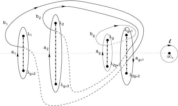
Figure 1. Homology cycles on $\Sigma$, adapted from [1]. The dashed vertical lines are branch cuts, the solid curves are portions of homology cycles on the upper sheet, the dashed curves are portions on the lower sheet, and the dotted horizontal line is the real axis in the $\lambda$-plane. Also shown are cycles $a_{g+1}$ and $\ell$, used in §§4 and 5.

Let $\omega_{1},\ ...\ \omega_{g}$ be holomorphic differentials on $\Sigma$, normalized as follows

$$\oint_{a_{k}}\omega_{j}=2\pi\mathrm{i}\delta_{jk},\qquad j,k=1,\ ...,\ g.$$

We introduce the period matrix $\mathcal{B}$ of entries

$$\mathcal{B}_{jk}=\oint_{b_{k}}\omega_{j},\qquad j,k=1,\ ...\ ,g,$$ (9)

and construct the associated Riemann theta function

$$\theta(\mathbf{z})=\sum_{\mathbf{n}\in{{\mathbb{Z}}}^{g}}\exp\left(\tfrac{1}{2}\langle\mathbf{n},\mathcal{B}\mathbf{n}\rangle+\langle\mathbf{n},\mathbf{z}\rangle\right),\quad\mathbf{z}\in{\mathbb{C}}^{g}.$$ (10)

The series (10) is absolutely convergent; this follows from the fact that $\operatorname{\sf Re}(\mathcal{B})$ is a negative definite matrix. Moreover, if $\mathbf{e}_{k}$’s are the standard basis vectors of ${\mathbb{C}}^{g}$ and $\mathbf{f}_{k}=\mathcal{B}\mathbf{e}_{k},$ for $k=1,\ldots g$, then

$$\theta(\mathbf{z}+2\pi\mathrm{i}\mathbf{e}_{k})=\theta(\mathbf{z}),\qquad\quad\theta(\mathbf{z}+\mathbf{f}_{k})=\mathrm{e}^{-\frac{1}{2}\mathcal{B}_{kk}-z_{k}}\theta(\mathbf{z});$$

in other words, $\theta$ is a quasi-periodic function. (The $\mathbf{e}_{k}$’s are called periods and the $\mathbf{f}_{k}$’s the quasiperiods of $\theta$.)

We also introduce the Abel map, which takes a divisor $\sum_{k=1}^{g}Q_{k}$ to a point of the complex torus $\operatorname{Jac}(\Sigma)={\mathbb{C}}^{g}/\Lambda$, where $\Lambda$ is the $2g$-dimensional lattice spanned by the columns of the matrix $({\textup{I}}\,|\mathcal{B})$. The Abel map of $\Sigma$ is defined by

$$\boldsymbol{\mathcal{A}}\,:\,\sum_{k=1}^{g}Q_{k}\longrightarrow\sum_{k=1}^{g}\int_{P_{0}}^{Q_{k}}\boldsymbol{\omega}\ \mathrm{mod}\Lambda,$$ (11)

where $P_{0}\in\Sigma$ is a given base point.

2.1. Eigenfunction formulas

The components of the vector-valued Baker-Akhiezer eigenfunction $\boldsymbol{\psi}$ are constructed in terms of ratios of Riemann theta functions:

$$\begin{split}\psi^{1}(P;s,t)=&\exp\left(\mathrm{i}s(\Omega_{1}(P)-\tfrac{E}{2})+\mathrm{i}t(\Omega_{2}(P)+\tfrac{N}{2})\right)\frac{\theta(\boldsymbol{\mathcal{A}}(P)+\mathrm{i}\mathbf{V}s+\mathrm{i}\mathbf{W}t-\boldsymbol{\mathcal{A}}({\mathcal{D}}_{+})-\boldsymbol{\mathcal{K}})}{\theta(\boldsymbol{\mathcal{A}}(P)-\boldsymbol{\mathcal{A}}({\mathcal{D}}_{+})-\boldsymbol{\mathcal{K}})}\\ &\times\frac{\theta(\boldsymbol{\mathcal{A}}(\infty_{-})-\boldsymbol{\mathcal{A}}({\mathcal{D}}_{+})-\boldsymbol{\mathcal{K}})}{\theta(\boldsymbol{\mathcal{A}}(\infty_{-})+\mathrm{i}\mathbf{V}s+\mathrm{i}\mathbf{W}t-\boldsymbol{\mathcal{A}}({\mathcal{D}}_{+})-\boldsymbol{\mathcal{K}})}\times\frac{g_{+}(P)}{g_{+}(\infty_{-})},\end{split}$$ (12)

and

$$\begin{split}\psi^{2}(P;s,t)=&\exp\left(\mathrm{i}s(\Omega_{1}(P)+\tfrac{E}{2})+\mathrm{i}t(\Omega_{2}(P)-\tfrac{N}{2})\right)\frac{\theta(\boldsymbol{\mathcal{A}}(P)+\mathrm{i}\mathbf{V}s+\mathrm{i}\mathbf{W}t-\boldsymbol{\mathcal{A}}({\mathcal{D}}_{-})-\boldsymbol{\mathcal{K}})}{\theta(\boldsymbol{\mathcal{A}}(P)-\boldsymbol{\mathcal{A}}({\mathcal{D}}_{-})-\boldsymbol{\mathcal{K}})}\\ &\times\frac{\theta(\boldsymbol{\mathcal{A}}(\infty_{+})-\boldsymbol{\mathcal{A}}({\mathcal{D}}_{-})-\boldsymbol{\mathcal{K}})}{\theta(\boldsymbol{\mathcal{A}}(\infty_{+})+\mathrm{i}\mathbf{V}s+\mathrm{i}\mathbf{W}t-\boldsymbol{\mathcal{A}}({\mathcal{D}}_{-})-\boldsymbol{\mathcal{K}})}\times\frac{g_{-}(P)}{g_{-}(\infty_{+})}.\end{split}$$ (13)

The ingredients of this formulas are described below:

1. The essential singularities of $\boldsymbol{\psi}$ at $\infty_{\pm}$ are introduced by means of the unique Abelian differentials $\mathrm{d}\Omega_{1}(P)$ and $\mathrm{d}\Omega_{2}(P),$ defined by their asymptotic expansions at $\infty_{\pm}$

   $$\mathrm{d}\Omega_{1}\sim\pm\mathrm{d}\lambda,\quad\mathrm{d}\Omega_{2}=\pm 4\lambda\,\mathrm{d}\lambda,\quad\text{as}\quad P\rightarrow\infty_{\pm},$$

   and normalized so that their integrals vanish along the $a$-cycles.

2. We will choose $P_{0}=\infty_{-}$ as basepoint for the Abel map $\boldsymbol{\mathcal{A}}$, and choose the rightmost branch point $\lambda_{2g+2}$ in the lower half-plane as basepoint for the Abelian integrals $\displaystyle\Omega_{j}(P)=\int_{\lambda_{2g+2}}^{P}\mathrm{d}\Omega_{j}$. This latter choice gives the property

   $$\Omega_{j}\circ\iota=-\Omega_{j},$$

   where $\iota:(\lambda,\mu)\mapsto(\lambda,-\mu)$ is the sheet interchange automorphism. In this way, the asymptotic expansions for $\Omega_{1}$ and $\Omega_{2}$ at $\infty_{\pm}$ are

   $$\Omega_{1}=\pm(\lambda-\tfrac{E}{2}+o(1))\quad{\rm and}\quad\Omega_{2}=\pm(2\lambda^{2}+\tfrac{N}{2}+o(1)),$$

   for certain constants $E$ and $N$.

3. Although they have different basepoints, we make the convention that the paths of integration for $\boldsymbol{\mathcal{A}}(P)$ and $\Omega_{j}(P)$ are yoked, so that a homology cycle may be added to one path only if it is added to the other; in other words, the difference between the paths for $\Omega_{j}(P)$ and $\boldsymbol{\mathcal{A}}(P)$ is a fixed path from $\infty_{-}$ to $\lambda_{2g+2}$. The most straightforward way of choosing this is to cut the Riemann surface along the homology cycles $a_{j},b_{j}$, resulting in a cut surface $\Sigma_{0}$ with boundary $\displaystyle\sum_{j}a_{j}+b_{j}-a_{j}-b_{j}$, and fixing a path $\Pi$ between $\infty_{-}$ and $\lambda_{2g+2}$ in the interior of $\Sigma_{0}$ (see Figure 2).

4. Then frequency vectors $\mathbf{V}$ and $\mathbf{W}$ are chosen to make $\psi^{1},\psi^{2}$ well-defined functions on $\Sigma$. In fact, if the paths of integration are modified by adding an integer linear combination $\sum_{k=1}^{g}n_{k}a_{k}+m_{k}b_{k}$ of homology cycles, then $\boldsymbol{\psi}$ changes by the factor

   $$\exp\left(\sum_{k=1}^{g}\left[m_{k}\left(\mathrm{i}s\oint_{b_{k}}\mathrm{d}\Omega_{1}+\mathrm{i}t\oint_{b_{k}}\mathrm{d}\Omega_{2}\right)-m_{k}\left(\mathrm{i}sV_{k}+\mathrm{i}tW_{k}\right)\right]\right),$$

   which equals $1$ if we define the components of $\mathbf{V}$ and $\mathbf{W}$ as

   $$V_{k}=\oint_{b_{k}}\mathrm{d}\Omega_{1},\qquad\qquad W_{k}=\oint_{b_{k}}\mathrm{d}\Omega_{2}.$$

5. ${\mathcal{D}}_{\pm}$ are the unique positive divisors linearly equivalent to ${\mathcal{D}}-\infty_{\pm}$, and $\boldsymbol{\mathcal{K}}$ is the vector of Riemann constants [12] which has the property that the zero divisor of $\theta({\boldsymbol{\mathcal{A}}}(P)-{\boldsymbol{\mathcal{A}}}(\mathcal{D}_{\pm})-\boldsymbol{\mathcal{K}})$ is ${\mathcal{D}_{\pm}}.$

6. In order to make $\psi^{1}$ and $\psi^{2}$ have pole divisor ${\mathcal{D}}$, the components of $\boldsymbol{\psi}$ are multiplied by meromorphic functions $g_{\pm}$ whose zero divisors are ${\mathcal{D}}_{\pm}+\infty_{\mp}$ and whose poles lie in the original divisor ${\mathcal{D}}$. For the sake of definiteness, we will normalize

   $$g_{+}(\infty_{-})=g_{-}(\infty_{+})=1.$$

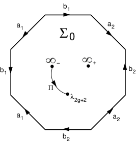
Figure 2. Cutting a two-hole torus $\Sigma$ along a homology basis, to yield the cut surface $\Sigma_{0}$

For later use (e.g., deriving formulas for the components of the VFE solution curve $\gamma$ given by (6)), we will explain how to derive a more compact and convenient expression for the eigenfunction. Let

$$\mathbf{D}=\boldsymbol{\mathcal{A}}(\mathcal{D}_{+})+\boldsymbol{\mathcal{K}},\qquad\qquad\qquad\mathbf{r}=\int_{\infty_{-}}^{\infty_{+}}\omega,$$

both computed using paths in $\Sigma_{0}$. Then $\boldsymbol{\mathcal{A}}(\mathcal{D}_{-})+\boldsymbol{\mathcal{K}}=\mathbf{D}+\mathbf{r}$, so

$$\psi^{1} =g_{+}(P)\exp\left(\mathrm{i}s(\Omega_{1}(P)-\tfrac{E}{2})+\mathrm{i}t(\Omega_{2}(P)+\tfrac{N}{2})\right)\dfrac{\theta(\boldsymbol{\mathcal{A}}(P)+\mathrm{i}\mathbf{V}s+\mathrm{i}\mathbf{W}t-\mathbf{D})\,\theta(\mathbf{D})}{\theta(\mathrm{i}\mathbf{V}s+\mathrm{i}\mathbf{W}t-\mathbf{D})\,\theta(\boldsymbol{\mathcal{A}}(P)-\mathbf{D})},$$

$$\psi^{2} =g_{-}(P)\exp\left(\mathrm{i}s(\Omega_{1}(P)+\tfrac{E}{2})+\mathrm{i}t(\Omega_{2}(P)-\tfrac{N}{2})\right)\dfrac{\theta(\boldsymbol{\mathcal{A}}(P)+\mathrm{i}\mathbf{V}s+\mathrm{i}\mathbf{W}t-\mathbf{D}-\mathbf{r})\,\theta(\mathbf{D})}{\theta(\mathrm{i}\mathbf{V}s+\mathrm{i}\mathbf{W}t-\mathbf{D})\,\theta(\boldsymbol{\mathcal{A}}(P)-\mathbf{D}-\mathbf{r})}.$$

Next, introduce another meromorphic differential $\mathrm{d}\Omega_{3}$, uniquely defined by

$$\mathrm{d}\Omega_{3}\sim\pm\dfrac{\mathrm{d}\lambda}{\lambda}\qquad\text{as}\ P\to\infty_{\pm},$$

and the requirement that it has zero $a$-periods. Let $\Omega_{3}(P)$ be the corresponding Abelian integral on $\Sigma$, computed with the same basepoint and convention for paths as $\Omega_{1}$,$\Omega_{2}$. Then, by imposing reality conditions that guarantee that the VFE solution is a curve in $\mathbb{R}^{3}$ at all times (see §5.2 for details), we obtain the following simplified expression for the components of $\boldsymbol{\psi}$:

$$\psi^{1} =\exp\left(\mathrm{i}s(\Omega_{1}(P)-\tfrac{E}{2})+\mathrm{i}t(\Omega_{2}(P)+\tfrac{N}{2})\right)\dfrac{\theta(\boldsymbol{\mathcal{A}}(P)+\mathrm{i}\mathbf{V}s+\mathrm{i}\mathbf{W}t-\mathbf{D})}{\theta(\mathrm{i}\mathbf{V}s+\mathrm{i}\mathbf{W}t-\mathbf{D})},$$ (14)

$$\psi^{2} =-\mathrm{i}\exp\left(\mathrm{i}s(\Omega_{1}(P)+\tfrac{E}{2})+\mathrm{i}t(\Omega_{2}(P)-\tfrac{N}{2})+\Omega_{3}(P)\right)\dfrac{\theta(\boldsymbol{\mathcal{A}}(P)+\mathrm{i}\mathbf{V}s+\mathrm{i}\mathbf{W}t-\mathbf{D}-\mathbf{r})}{\theta(\mathrm{i}\mathbf{V}s+\mathrm{i}\mathbf{W}t-\mathbf{D})}.$$ (15)

An explicit computation involving the asymptotic expansions of the eigenfunction $\boldsymbol{\psi}$ at $\infty_{\pm}$ (see, e.g., [1]) shows that $\boldsymbol{\psi}$ is a common solution of the pair of NLS linear systems (4) with potential $q$ given by

$$q(x,t)=A\exp(-\mathrm{i}Es+\mathrm{i}Nt)\dfrac{\theta(\mathrm{i}\mathbf{V}s+\mathrm{i}\mathbf{W}t-\mathbf{D}+\mathbf{r})}{\theta(\mathrm{i}\mathbf{V}s+\mathrm{i}\mathbf{W}t-\mathbf{D})},$$ (16)

where the formula for the constant $A$ is given in §5.2.

2.2. Curve Formulas

When $\pi(P)$ is real, a fundamental solution matrix of (4) is given by

$$\Psi(P;s,t)=\left(\begin{array}[]{cc}\psi^{1}(P)&-\overline{\psi^{2}(P)}\\ \psi^{2}(P)&\overline{\psi^{1}(P)}\end{array}\right).$$ (17)

The Sym-Pohlmeyer reconstruction formula (5) yields the following expression for the components of the skew-hermitian matrix $\Gamma$ representing the position vector of the VFE solution:

$$\Gamma_{11} =i(\Omega^{\prime}_{(}P)s+\Omega^{\prime}_{2}(P)t)$$ (18)

$$+\dfrac{1}{2\det\Psi}\left[|\psi^{1}|^{2}\nabla\log\left(\dfrac{\theta(\boldsymbol{\mathcal{A}}(P)+\boldsymbol{\varphi})}{\theta(\boldsymbol{\mathcal{A}}(P)-\boldsymbol{\varphi})}\right)+|\psi^{2}|^{2}\nabla\log\left(\dfrac{\theta(\boldsymbol{\mathcal{A}}(P)+\boldsymbol{\varphi}-\mathbf{r})}{\theta(\boldsymbol{\mathcal{A}}(P)-\boldsymbol{\varphi}-\mathbf{r})}\right)\right]\cdot\dfrac{\mathrm{d}\boldsymbol{\mathcal{A}}(P)}{\mathrm{d}\lambda},$$

$$\Gamma_{21} =\dfrac{\psi^{1}\psi^{2}}{\det\Psi}\left(\nabla\log\left(\dfrac{\theta(\boldsymbol{\mathcal{A}}(P)+\boldsymbol{\varphi}-\mathbf{r})}{\theta(\boldsymbol{\mathcal{A}}(P)+\boldsymbol{\varphi})}\right)\cdot\dfrac{\mathrm{d}\boldsymbol{\mathcal{A}}(P)}{\mathrm{d}\lambda}+\Omega^{\prime}_{3}(P)\right),$$

where $\boldsymbol{\varphi}=\mathrm{i}\mathbf{V}s+\mathrm{i}\mathbf{W}t-\mathbf{D}$, and $\Omega^{\prime}_{j}(P)=\mathrm{d}\Omega_{j}(P)/\mathrm{d}\lambda$.

It is easy to verify that, given a fundamental solution matrix $\Psi$ of the linear systems (4), the quantity $\det{\Psi}=|\psi^{1}|^{2}+|\psi^{2}|^{2}$ is independent of both $s$ and $t$. Differentiating it with respect to $s$, one gets

$$\left[|\psi^{1}|^{2}\nabla\log\left(\dfrac{\theta(\boldsymbol{\mathcal{A}}(P)+\boldsymbol{\varphi})}{\theta(\boldsymbol{\mathcal{A}}(P)-\boldsymbol{\varphi})}\right)+|\psi^{2}|^{2}\nabla\log\left(\dfrac{\theta(\boldsymbol{\mathcal{A}}(P)+\boldsymbol{\varphi}-\mathbf{r})}{\theta(\boldsymbol{\mathcal{A}}(P)-\boldsymbol{\varphi}-\mathbf{r})}\right)-2\det\Psi\nabla\log\theta(\boldsymbol{\varphi})\right]\cdot\mathbf{V}=0.$$

Differentiation with respect to $t$ yields a similar identity with $\mathbf{V}$ replaced by $\mathbf{W}$. Since the two frequency vectors span $\mathbb{C}^{2}$, one concludes that the quantity between the square brackets must vanish and obtains the following

Proposition 2.3.

The components $(\gamma_{1},\gamma_{2},\gamma_{3})$ of the position vector ${\boldsymbol{\gamma}}$ of an N-phase solution of the Vortex Filament Equation are given by the following expressions

$$\Gamma_{21}=\gamma_{1}+\mathrm{i}\gamma_{2} =\dfrac{\psi^{1}\psi^{2}}{\det\Psi}\left(\nabla\log\left(\dfrac{\theta(\boldsymbol{\mathcal{A}}(P)+\mathrm{i}\mathbf{V}s+\mathrm{i}\mathbf{W}t-\mathbf{D}-\mathbf{r})}{\theta(\boldsymbol{\mathcal{A}}(P)+\mathrm{i}\mathbf{V}s+\mathrm{i}\mathbf{W}t-\mathbf{D})}\right)\cdot\dfrac{d\boldsymbol{\mathcal{A}}(P)}{d\lambda}+\Omega^{\prime}_{3}(P)\right),$$

$$\Gamma_{11}=\gamma_{3} =\mathrm{i}[\Omega^{\prime}_{1}(P)s+\Omega^{\prime}_{2}(P)t]+\nabla\log\theta(\mathrm{i}\mathbf{V}s+\mathrm{i}\mathbf{W}t-\mathbf{D})\cdot\dfrac{d\boldsymbol{\mathcal{A}}(P)}{d\lambda},$$

where $\pi(P)=\Lambda_{0}\in{\mathbb{R}}$ is the reconstruction point.

2.3. Closure Conditions

The potential $q$ associated with a closed curve of length $L$ by the Hasimoto map is $L$-periodic, but only up to multiplication by a unit modulus constant:

$$q(s+L)=e^{\mathrm{i}\phi}q(s),\qquad\text{where\ }\phi=\int_{0}^{L}\tau\,ds.$$

However, a quasiperiodic potential like this is related to a genuinely periodic NLS solution by the NLS symmetry mentioned in the introduction:

$$\tilde{q}(s,t)=\mathrm{e}^{\mathrm{i}(as-a^{2}t)}q(s-2at,t).$$

(Obviously, one chooses $a=-\phi/L$ to make $\tilde{q}$ a periodic potential.) This symmetry lifts to the NLS linear system:

$$\boldsymbol{\psi}(s,t;\tilde{q},\tilde{\lambda})=\exp(\tfrac{\mathrm{i}}{2}(as-a^{2}t)\sigma_{3})\boldsymbol{\psi}(s-2at,t;q,\lambda),\qquad\text{where}\ \tilde{\lambda}=\lambda-\tfrac{1}{2}a.$$

(This transformation, for fixed time $t=0$, appears in Grinevich and Schmidt [16].) It follows that the continuous spectrum of $\tilde{q}$ is the same as that of $q$, but translated by $-a/2$, and the Sym formula (6) yields the same curves at corresponding values of $\lambda$:

$$\Gamma|_{\lambda=\Lambda_{0}}=\tilde{\Gamma}|_{\tilde{\lambda}=\Lambda_{0}-\frac{1}{2}a}.$$

Thus, we can without loss of generality assume that a closed curve of length $L$ is generated from a potential $q(s,t)$ that is $L$-periodic in the variable $s$. Note that, for finite-gap solutions, the value of the frequency vector $\mathbf{V}$ is unchanged under horizontal translation $\lambda_{j}\mapsto\lambda_{j}-\frac{1}{2}a$ of the branch points, but the phase constant $E$ changes by $E\mapsto E-a$. In fact, our assumption that $q$ is $L$-periodic implies that $E$ has been translated to zero and the entries of $\mathbf{V}$ are rational multiples of $2\pi/L$. Therefore, if $V$ is the greatest common divisor of the entries of $\mathbf{V}$, then $q$ has period $T=2\pi/V$, and $L$ is an integer multiple of $T$.

Since the natural curvatures (which are one half the real and imaginary parts of $q(s,t)$) are periodic, the corresponding natural frame vectors must also be periodic. Since those are obtained by conjugating a fixed basis of ${\mathfrak{su}}(2)$ by the fundamental matrix $\Psi$, it follows that $\Psi$ must be $L$-periodic or antiperiodic. For finite-gap solutions satisfying the periodicity condition, this amounts to assuming that $\Omega_{1}(P)$ is an integer multiple of $\pi/L$.

Examining the formulas (18) shows that our assumptions so far guarantee that $\Gamma_{21}$ is periodic, and that $\Gamma_{11}$ is periodic if and only if $\mathrm{d}\Omega_{1}(P)$ vanishes. We summarize these closure conditions as:

Proposition 2.4 (Closure).

Suppose $q(s,t)$ is a finite-gap potential of period $2\pi/V$ in $s$. Then the curve reconstructed from $q$ using the Sym formula (6) with $\Lambda_{0}=\lambda(P)$ is smoothly closed of length $L=2n\pi/V$ if and only if (a) $\mathrm{d}\Omega_{1}(P)=0$ and (b) $\exp(\mathrm{i}L\Omega_{1}(P))=\pm 1$.

The points which fulfil the closure condition (b) are discrete points of the Floquet spectrum associated with the potential $q$, which can be described in terms of Floquet discriminant. The Floquet discriminant of $q$ is defined as the trace of the transfer matrix of $\Psi$ over the interval $[0,L]$:

$$\Delta(q;\lambda)=\operatorname{tr}\left(\Psi(s,t;\lambda)^{-1}\Psi(s+L,t;\lambda)\right).$$

(Because the transfer matrix only changes by conjugation when we shift in $s$ or $t$, $\Delta$ is independent of those variables.) Then, the Floquet spectrum is defined as the region

$$\sigma(q)=\{\lambda\in\mathbb{C}\,|\,\Delta(q;\lambda)\in\mathbb{R},-2\leq\Delta\leq 2\}.$$

Points of the continuous spectrum of $q$ are those for which the eigenvalues of the transfer matrix have unit modulus, and therefore $\Delta(q;\lambda)$ is real and between $2$ and $-2$; in particular, the real line is part of the continuous spectrum. Points of the $L$-periodic discrete spectrum of $q$ are those for which the eigenvalues of the transfer matrix are $\pm 1$, equivalently $\Delta(q;\lambda)=\pm 2$. Points of the discrete spectrum which are embedded in a continuous band of spectrum have to be critical points for the Floquet discriminant (i.e., $\mathrm{d}\Delta/\mathrm{d}\lambda$ must vanish at such points); thus, the conditions in Proposition 2.4 may be rephrased as requiring $\Lambda_{0}$ to be a real zero of the quasimomentum differential that is also a double point. These conditions coincide with those derived by Grinevich and Schmidt [16] using different reasoning.

For finite-gap potentials, we may use the simplified eigenfunction formulas (14),(15) to write the Floquet discriminant as

$$\Delta(q;\lambda)=2\cos(L\Omega_{1}(P)),\qquad\lambda=\pi(P).$$

If we have an explicit formula for the discriminant, we can use it to locate the points of the discrete spectrum; see §3.5 for an example. However, it is very difficult, in general, to determine how to choose the branch points so that a point of the discrete spectrum coincides with a zero of the quasimomentum differential. Even in genus one, this corresponds to an implicit equation involving elliptic integrals.

2.4. Periodic Self-Intersection

Whether or not the filament closes smoothly, it may intersect itself after one period $T$ of the potential. (For example, this happens with elastic rod centerlines [20].) In this section, we will calculate the general condition under which this happens. In the expression for $\Gamma_{11}$ in (18), the only term which is not automatically $T$-periodic is the linear term $\mathrm{i}\Omega^{\prime}_{1}(P)s$. Therefore, $\Gamma_{11}$ is $T$-periodic if and only if $\Omega^{\prime}_{1}(P)=0$, i.e., the first condition of Prop. 2.4 above is satisfied. So, we will assume this condition. Next, $\Gamma_{21}$ is $T$-periodic if and only if

$$\psi^{1}\psi^{2}=-\mathrm{i}\exp(2\mathrm{i}(\Omega_{1}(P)s+\Omega_{2}(P)t)+\Omega_{3}(P))\dfrac{\theta(\boldsymbol{\mathcal{A}}(P)+\boldsymbol{\varphi})\theta(\boldsymbol{\mathcal{A}}(P)+\boldsymbol{\varphi}-\mathbf{r})}{\theta(\boldsymbol{\varphi})^{2}}$$

is periodic. But that amounts to assuming that $\lambda(P)$ is a point for the $T$-periodic discrete spectrum, giving a smoothly closed filament of length $T$. However, self-intersection may also occur if the last factor in $\Gamma_{21}$ vanishes for some $s$-value:

$$\left.\nabla\log\left(\dfrac{\theta(\boldsymbol{\mathcal{A}}(P)+\boldsymbol{\varphi}-\mathbf{r})}{\theta(\boldsymbol{\mathcal{A}}(P)+\boldsymbol{\varphi})}\right)\cdot\dfrac{d\boldsymbol{\mathcal{A}}(P)}{d\lambda}\right|_{s=s_{0}}+\Omega^{\prime}_{3}(P)=0.$$ (19)

(Note that this factor is also $T$-periodic in $s$.) Then $\Gamma_{21}$ is not $T$-periodic, but is equal to zero at a succession of $s$-values, and the $T$-periodicity of $\Gamma_{11}$ guarantees that the filament returns to the same point in ${\mathbb{R}}^{3}$.

For finite-gap solutions, the first self-intersection condition $\Omega^{\prime}_{1}(P)=0$ is polynomial in $\lambda$. In general, the second condition (19) depends on $\lambda,s_{0}$ and also $t$, so that this kind of self-intersection may only be present at one time. However, in genus one, a shift in time may be offset by a shift in $s_{0}$, so that these self-intersections persist in time. Furthermore, in genus one the derivatives of the logarithms may be expressed in terms of Jacobi zeta functions, and we may choose $s_{0}$ and $t$ to give $\boldsymbol{\varphi}=0$. This yields a polynomial condition in $\lambda$. We conjecture that an analogous polynomial condition occurs in higher genus.

3. Genus One Solutions

In this section, we will work out the representation of solutions of the filament flow in detail for the case when the genus is one, when $\Sigma$ is an elliptic curve given by the equation

$$\mu^{2}=\prod_{j=1}^{2g+2}(\lambda-\lambda_{j})=(\lambda-\lambda_{1})(\lambda-\lambda_{2})(\lambda-\overline{\lambda}_{1})(\lambda-\overline{\lambda}_{2}).$$ (20)

The Floquet spectrum of a generic $2$-phase solution is shown in Figure 5(a). In particular, the intersection points $\alpha_{1}$ and $\alpha_{2}$ of the complex bands of spectrum with the real axis are the real zeros of the quasimomentum differential $\mathrm{d}\Omega_{1}$ given in equations (36),(38) below. As discussed earlier, closed curves are obtained by selecting the branch points $\lambda_{j}$ so that one of the $\alpha_{j}$ is also a double point, and using $\Lambda_{0}=\alpha_{j}$ in the reconstruction formula (6).

3.1. Elastic Rods

Filaments generated by genus one potentials are interesting objects from geometric and topological points of view, because they are the centerlines for Kirchhoff elastic rods. These are thin rods that are critical for an energy that consists of one term for the isotropic bending energy (i.e., a multiple of $\int\kappa^{2}ds$, where $\kappa$ is the Frenet curvature of the centerline) and a term for the twisting of the rod about its centerline. Solutions of this physical variational problem are exactly the solutions of a geometric variational problem, where the Lagrangian is of the form

$${\mathcal{F}}=\int\tfrac{1}{2}\kappa^{2}\,\mathrm{d}s+l_{1}\int\tau\,\mathrm{d}s+l_{2}\int\mathrm{d}s.$$ (21)

(The values of the parameters $l_{1},l_{2}$ depending both on the relative weight of the bending and twisting energies and on the boundary conditions in the physical variational problem; see [20] and [27] for details.) Regarding $l_{1},l_{2}$ as Lagrange multipliers, we can think of Kirchhoff elastic rod centerlines as extremizing the bending energy subject to constant total torsion and constant length constraints. These curves include classical Eulerian elastic curves (for $l_{1}=0$) and free elastica (for $l_{1}=l_{2}=0$).

The identification between travelling wave solutions of the NLS and elastic rod centerlines was first discovered by Kida [22], who sought solutions of the filament flow that moved by rigid motion (i.e., rotation and/or translation) plus possibly a translation along the curve. (As we will see below, under the Hasimoto map these filaments correspond exactly to finite-gap NLS potentials of genus one.) Kida obtained parametrizations for such curves, in terms of elliptic integrals, showed that there exist smooth closed curves of this type, and identified the planar curves of this type with Eulerian elastica.

Later, Langer and Singer [27] began with the variational problem for ${\mathcal{F}}$ above, and showed that solutions were precisely those curves which move by rigid motion (plus translation along the curve) under the filament flow. Langer and Singer expressed the curvature and torsion of these curves in terms of periodic elliptic functions; consequently, these curves consist of repeated congruent segments which smoothly close up if certain elliptic integrals satisfy a rationality condition. Figure 3 shows some examples.

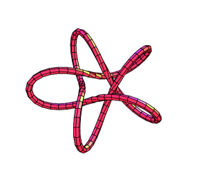
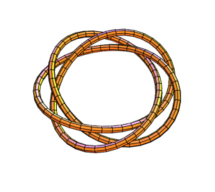
Figure 3. Some examples of knotted elastic rods.

Like these specimens, all closed elastic rod centerlines have discrete rotational symmetry about an axis. It is not hard to see that if such a curve is knotted, it must be a torus knot. Ivey and Singer [20] later showed that every torus knot type is realized by a one-parameter family of smooth elastic rod centerlines. In fact, each such family connects smoothly to another family of centerlines with the same rotational symmetry, but with a complementary torus knot type (like $(2,5)$ and $(-3,5)$ shown above). We call this a homotopy of closed elastic rod centerlines.

3.2. Genus One Potentials

We now turn to the detailed calculation of genus one NLS potentials. The data necessary to construct $q$ will be expressed in terms of elliptic integrals and algebraic functions of the branch points. For these calculations, we rely heavily on the treatise by Byrd and Friedman [4]; citations of the form “formula xxx.yy” refer to this volume.

We begin by choosing a standard homology basis $a,b$ on the elliptic curve $\Sigma$ (see Figure 4) and computing the periods of holomorphic differentials.

Figure 4. Branch points for elliptic curve $\Sigma$ with oriented homology cycles and branch cuts. The upper sheet tends to $\infty_{+}$ to the right and left.

Lemma 3.1.

$$\oint_{a}\frac{\mathrm{d}\lambda}{\mu}=\frac{4\mathrm{i}K}{|\lambda_{1}-\overline{\lambda}_{2}|},\qquad\oint_{b}\frac{\mathrm{d}\lambda}{\mu}=\frac{-4K^{\prime}}{|\lambda_{1}-\overline{\lambda}_{2}|},$$ (22)

where we introduce the abbreviations

$$K:=K(p),\qquad K^{\prime}:=K(p^{\prime})$$

for complete elliptic integrals of the first kind with moduli

$$p^{\prime}:=\dfrac{|\lambda_{1}-\lambda_{2}|}{|\lambda_{1}-\overline{\lambda}_{2}|},\qquad p:=\sqrt{1-(p^{\prime})^{2}}.$$

Proof.

We will give a somewhat detailed explanation of this calculation, since it is a model for others below.

To transform the integrals in (22) to elliptic integrals along the real axis, we use the linear fractional substitution

$$\lambda(x)=\overline{\lambda}_{2}+\dfrac{\lambda_{2}-\overline{\lambda}_{2}}{1-hx},\qquad h:=\dfrac{\lambda_{1}-\lambda_{2}}{\lambda_{1}-\overline{\lambda}_{2}},$$ (23)

under which $\lambda_{1},\overline{\lambda}_{1},\lambda_{2},\overline{\lambda}_{2}$ correspond to $x$-values $1,(p^{\prime})^{-2},0,\infty$ respectively. Then (20) gives

$$\mu^{2}=-h^{2}|\lambda_{1}-\overline{\lambda}_{2}|^{2}\left(\dfrac{\lambda_{2}-\overline{\lambda}_{2}}{1-hx}\right)^{2}\left(x(x-1)(1-(p^{\prime})^{2}x)\right).$$ (24)

Without changing the value of the $a$-integral in (22), the $a$-cycle may be contracted in the $\lambda$-plane to a straight-line path that travels on the left-hand edge of the branch cut, from $\overline{\lambda}_{1}$ to $\lambda_{1}$, and then back along the right-hand edge of the branch cut. Since $\mu$ differs only by a minus sign on the two sides of the branch cut, the $a$-integral is twice the integral along the left-hand edge, where ${\sf Re}(\mu)>0$. As $\lambda$ moves along this path, $x$ moves from $(p^{\prime})^{-2}$ to $1$. Thus ${\sf Im}(\mathrm{d}\lambda)>0$ and ${\sf Re}(dy)<0$ as we move along this path, so the equation

$$\mathrm{d}\lambda=\dfrac{h(\lambda_{2}-\overline{\lambda}_{2})}{1-hy}dy$$

shows that ${\sf Re}(h/(1-hy))<0$ there. Hence, along this path we take

$$\mu=|(\lambda_{1}-\overline{\lambda}_{2})(\lambda_{2}-\overline{\lambda}_{2})|\left(\dfrac{-h}{1-hy}\right)\sqrt{x(x-1)(1-(p^{\prime})^{2}x)},$$

giving

$$\frac{1}{2}\oint_{a}\dfrac{\mathrm{d}\lambda}{\mu}=\dfrac{-2\mathrm{i}}{|\lambda_{1}-\overline{\lambda}_{2}|}\int_{(p^{\prime})^{-2}}^{1}\dfrac{dy}{\sqrt{x(x-1)(1-(p^{\prime})^{2}x)}}.$$

Reversing the limits in the integral on the right-hand side yields the complete elliptic integral $K(p)$ (see formula 236.00).

The computation of the $b$-integral is similar. ∎

Consequently, the normalized holomorphic differential (with $a$-period equal to $2\pi\mathrm{i}$) is

$$\omega=2\pi\mathrm{i}\left(\dfrac{|\lambda_{1}-\overline{\lambda}_{2}|}{4\mathrm{i}K}\right)\dfrac{\mathrm{d}\lambda}{\mu},$$

and the ‘Riemann matrix’ for the $\theta$-function used in the construction of $q$ is

$$B=\oint_{b}\omega=-2\pi K^{\prime}/K,$$ (25)

The frequencies inside the $\theta$-function are

$$V=4\pi\mathrm{i}\left(\oint_{a}\mathrm{d}\lambda/\mu\right)^{-1}=\pi|\lambda_{1}-\overline{\lambda}_{2}|/K$$

and $W=cV$, where

$$c=\sum_{j=1}^{2g+2}\lambda_{j}=\lambda_{1}+\overline{\lambda}_{1}+\lambda_{2}+\overline{\lambda}_{2}.$$ (26)

Using the formulas (64),(65), the frequencies in the exponential part of $q$ are given by

$$E=c-2L,\qquad N=2cL-4d-c^{2},$$

where $c$ is as in (26), $d$ is given by (63), and $L$ is the following ratio of $a$-periods:

$$L:=\left.\oint_{a}\dfrac{\lambda}{\mu}\mathrm{d}\lambda\right/\oint_{a}\dfrac{\mathrm{d}\lambda}{\mu}.$$

To calculate the numerator of $L$, we use the same path and change of variables as in the proof of Lemma 3.1. Thus, along the left edge of the branch cut, we have

$$\dfrac{\lambda}{\mu}\mathrm{d}\lambda=\dfrac{-\mathrm{i}}{|\lambda_{1}-\overline{\lambda}_{2}|}\left(\overline{\lambda}_{2}+\dfrac{\lambda_{2}-\overline{\lambda}_{2}}{1-hx}\right)\dfrac{dy}{\sqrt{x(x-1)(1-(p^{\prime})^{2}x)}}.$$

Applying formula 236.02, we get

$$L=\overline{\lambda}_{2}+(\overline{\lambda}_{1}-\overline{\lambda}_{2})\dfrac{\Pi(\beta^{2},p)}{K},$$ (27)

where $\Pi(\beta^{2},p)$ denotes a complete elliptic integral of the third kind, with parameter

$$\beta^{2}:=\dfrac{p^{2}}{1-\overline{h}}=\dfrac{\lambda_{1}-\overline{\lambda}_{1}}{\lambda_{1}-\overline{\lambda}_{2}}.$$

Note that we may also calculate $L$ using formula 235.02, obtaining

$$L=\lambda_{2}+(\lambda_{1}-\lambda_{2})\dfrac{\Pi(\overline{\beta}^{2},p)}{K}.$$ (28)

This is equivalent to (27) by application of the addition formula 117.03 for elliptic integrals of the third kind. Furthermore, comparing (27) and (28) shows that $L$ is real, as it must be since complex conjugation

$$\tau:(\lambda,\mu)\mapsto(\overline{\lambda},\overline{\mu})$$

takes cycle $a$ to $-a$.

To calculate the shift $r$ in (16), we use the Abelian differential

$$\mathrm{d}\Omega_{3}=\dfrac{\lambda-L}{\mu}\mathrm{d}\lambda$$

which has $a$-period equal to zero. Using formula 233.02 to compute $\oint_{b}(\lambda/\mu)\mathrm{d}\lambda$ gives

$$r=-\oint_{b}\mathrm{d}\Omega_{3}=\dfrac{4}{|\lambda_{1}-\overline{\lambda}_{2}|}\left[(\overline{\lambda}_{2}-L)K^{\prime}+(\lambda_{2}-\overline{\lambda}_{2})\Pi(h,p^{\prime})\right].$$ (29)

One can verify that ${\sf Im}(r)=\pi$ by using the addition formula 117.02 to simplify $\Pi(h,p)+\Pi(\overline{h},p)$, given that $\overline{h}=(p^{\prime})^{2}/h$.

It will later be convenient to have an alternate formula for $r$. Using addition formula 117.05, we can write

$$(1-h)K\left(\Pi(h,p^{\prime})-K^{\prime}\right)=hK^{\prime}\Pi(\overline{\beta}^{2},p)-\dfrac{\pi}{2}\sqrt{\dfrac{1-h}{\overline{h}-1}}F(\phi,p^{\prime}),\qquad\phi=\arcsin\left(\sqrt{h}/p^{\prime}\right),$$

where $F$ denotes an incomplete elliptic integral of the first kind, e.g., $F(\pi/2,p^{\prime})=K^{\prime}$. (Note that $|h|=(p^{\prime})^{2}<1$, $\arg(h)\in[0,\pi)$, $\arg\left((1-h)/(\overline{h}-1)\right)=2\arg(\lambda_{2}-\overline{\lambda}_{1})\in(0,\pi)$, and we take the square root to have positive real part.) We use this formula to substitute for $\Pi(h,p^{\prime})$ in (29), and use (28) to substitute for $L$, to get

$$r=\dfrac{2\pi}{K}F(\phi,p^{\prime})$$ (30)

Finally, the modulus of scalar $A$ may be calculated by numerical integration as described in Appendix 5.3. However, we also have the following formula,

$$|A|=\dfrac{|\lambda_{1}-\overline{\lambda}_{2}|}{\theta(r)}\sqrt{\dfrac{2pp^{\prime}K}{\pi}},$$ (31)

which may be derived by substituting the formula (16) for the potential into the NLS and evaluating at $s=t=0$.

3.3. Geometric Interpretation

The above information is enough to enable us to discuss the geometric invariants (i.e., curvature and torsion) for the filaments corresponding to a genus one potential $q(s,t)$.

Because a translation in time modifies $q$ only by a unit modulus factor which is independent of $s$, and may be absorbed inside the theta function by translation in $s$, the geometric invariants at time $t$ differ from those at time zero only by a constant-speed translation in $s$. Thus, the filament at time $t$ is obtained from the filament at time zero by Euclidean motions (accompanied by a translation along the curve). It follows from the semigroup property of the evolution equation that the Euclidean motions must belong to a one-parameter subgroup. Together with the discussion at the beginning of this section, this gives the following

Proposition 3.2.

All finite-gap solutions of genus one for the vortex filament equation move by rigid motions, and are congruent to elastic rod centerlines.

It is instructive to express the curvature of genus one solutions in terms of elliptic functions. By the above argument, we may assume that $t=0$ without loss of generality. Also, since the reality condition (see Appendix 5.2) implies that $D$ is purely imaginary, we may assume that $D=0$.

We first observe that for $B$ given by (25),

$$\theta(2\mathrm{i}z)=\theta_{3}(z)=\theta_{0}(z+\pi/2),$$

where $\theta_{k}$ denotes the Jacobi theta function with modulus $p$ and period $2\pi$ (for $k=1,2$) or $\pi$ (for $k=0,3$). Next, let $\rho=\frac{1}{2}{\sf Re}(r)$. Then

$$q(s,0)=A\exp(-\mathrm{i}Es)\dfrac{\theta_{3}((Vs+\pi)/2-\mathrm{i}\rho)}{\theta_{0}((Vs+\pi)/2).}$$ (32)

For convenience, introduced the rescaled variable $z=(Vx+\pi)/2$. Then, using the translation properties and addition formulas 1051.ff for Jacobi theta functions, we have

$$\kappa^{2}=|2q(s,0)|^{2}=|2A|^{2}\dfrac{\theta_{3}(z+\mathrm{i}\rho)\theta_{3}(z-\mathrm{i}\rho)}{\theta_{0}^{2}(z)}=|2A|^{2}\dfrac{\theta_{3}^{2}(\mathrm{i}\rho)}{\theta_{0}^{2}(0)}\left(1-\dfrac{\theta_{2}^{2}(\mathrm{i}\rho)\theta_{1}^{2}(z)}{\theta_{3}^{2}(\mathrm{i}\rho)\theta_{0}^{2}(z)}\right).$$

This formula coincides with the curvature formula for elastic rod centerlines derived in [27]; for, if we set

$$w:=\operatorname{dc}(2Ki\rho/\pi)=\operatorname{dn}(2K\rho/\pi,p^{\prime}),$$ (33)

and substitute in for $|A|$ from (31), then we have

$$\kappa^{2}=\kappa_{0}^{2}\left(1-\dfrac{p^{2}}{w^{2}}\operatorname{sn}^{2}u\right),\qquad\text{where}\qquad u=\dfrac{2K}{\pi}z=\dfrac{\kappa_{0}}{2w}(s+\pi/V),$$

and we use $\kappa_{0}=2w|\lambda_{1}-\overline{\lambda}_{2}|$ to denote the maximum curvature.

We will now make some specific observations about the relation between the geometry of the filament and the spectrum in genus one. For these, we will need the following formula:

Lemma 3.3.

$$w^{2}=\dfrac{|{\sf Im}(\lambda_{1}-\overline{\lambda}_{2})|^{2}}{|\lambda_{1}-\overline{\lambda}_{2}|^{2}}$$ (34)

Proof.

Using (30), we compute that

$$w=\operatorname{dn}(2K\rho/\pi,p^{\prime})=\mathrm{i}\operatorname{cs}(Kr/\pi,p^{\prime})=\mathrm{i}\operatorname{cn}(2F,p^{\prime})/\operatorname{sn}(2F,p^{\prime}),$$

where $F=F(\phi,p^{\prime})$, as in (30). Then, using double angle formulas 124.01,

$$w=\dfrac{\operatorname{sn}^{2}(F,p^{\prime})\operatorname{dn}^{2}(F,p^{\prime})-\operatorname{cn}^{2}(F,p^{\prime})}{2\mathrm{i}\operatorname{sn}(F,p^{\prime})\operatorname{cn}(F,p^{\prime})\operatorname{dn}(F,p^{\prime})}=\pm\dfrac{{\sf Re}(h-1)}{|h-1|},$$

where the ambiguity of sign arises from solving $\operatorname{sn}(F,p^{\prime})=\sqrt{h}/p^{\prime}$ for the values of $\operatorname{cn}(F,p^{\prime})$ and $\operatorname{dn}(F,p^{\prime})$. Then substituting (23) yields the result. ∎

In [27], it is shown that the curvature and torsion of an elastic rod centerline satisfy

$$2\tau-l_{1}=j/\kappa^{2},\quad\text{where}\quad j^{2}=\dfrac{\kappa_{0}^{6}}{w^{4}}(1-w^{2})(w^{2}-p^{2}),$$ (35)

and $l_{1}$ is the ratio of the coefficient of the term $\int\tau\,ds$ to the coefficient of the elastic energy $\int\tfrac{1}{2}\kappa^{2}\,ds$ in the Lagrangian (21). It is clear that the torsion of the centerline is constant if and only if $w^{2}=p^{2}$ or $w^{2}=1$. From (34) we see that these correspond to the cases where $\lambda_{1}-\lambda_{2}$ is purely real or purely imaginary, respectively. In these cases, we may translate the branch points so that they are symmetric under the reflection $\lambda\mapsto-\lambda$ about the origin. (Recall that the curve produced by the Sym-Pohlmeyer formula is unchanged provided we apply the same translation to the reconstruction point $\Lambda_{0}$.) We summarize these observations:

Proposition 3.4.

A filament associated to a finite-gap solution of genus one has constant torsion if and only the branch points are symmetric about an axis perpendicular to the real axis.

In §4 of this paper, we will discuss what symmetry of the branch points means in higher genus.

3.4. Quasimomentum Differential

Before making further observations, we need to calculate the meromorphic differential $\mathrm{d}\Omega_{1}$ for genus one. (Recall that the zeros $\alpha_{k}$ of this differential are used to reconstruct closed curves.) This will later enable us to calculate the Floquet discriminant, and (in Prop. 3.5 below) to connect the coalescence of the $\alpha_{k}$’s with the filament being an elastic curve.

The form of this differential is

$$\mathrm{d}\Omega_{1}=\dfrac{\lambda^{2}-\tfrac{c}{2}\lambda-c_{1}}{\mu}\,\mathrm{d}\lambda,$$ (36)

where $c$ is as in (26) and $c_{1}$ is chosen so that the $a$-period of $\mathrm{d}\Omega_{1}$ is zero. The value of $\oint_{a}(\lambda/\mu)\mathrm{d}\lambda$ was obtained in the above calculation of $L$. In a similar way, we apply formulas 236.17 and 336.02 to get

$$\oint_{a}\dfrac{\lambda^{2}}{\mu}\mathrm{d}\lambda=\dfrac{4\mathrm{i}}{|\lambda_{1}-\overline{\lambda}_{2}|}\left[\overline{\lambda}_{2}^{2}K+2\overline{\lambda}_{2}(\overline{\lambda}_{1}-\overline{\lambda}_{2})\Pi(\beta^{2},p)\right.\\ +\left.\dfrac{(\overline{\lambda}_{1}-\overline{\lambda}_{2})^{2}}{2(1-\beta^{2})(\beta^{2}-p^{2})}\left(\beta^{2}E(p)+(p^{2}-\beta^{2})K+(2\beta^{2}p^{2}+2\beta^{2}-\beta^{4}-3p^{2})\Pi(\beta^{2},p)\right)\right],$$ (37)

where $E(p)$ is the complete elliptic integral of the second kind. We combine the previous two results to compute

$$c_{1}=\left.\oint_{a}\dfrac{\lambda^{2}-\tfrac{c}{2}\lambda}{\mu}\mathrm{d}\lambda\right/\oint_{a}\dfrac{\mathrm{d}\lambda}{\mu}.$$

Miraculously, the coefficient of $\Pi(\beta^{2},p)$ in $c_{1}$ is zero, giving

$$\mathrm{d}\Omega_{1}=\left[\lambda^{2}-\tfrac{c}{2}\lambda-\tfrac{1}{2}\left(|\lambda_{1}-\overline{\lambda}_{2}|^{2}\dfrac{E(p)}{K}-|\lambda_{1}|^{2}-|\lambda_{2}|^{2}\right)\right]\dfrac{\mathrm{d}\lambda}{\mu}.$$ (38)

The roots of the quadratic polynomial in $\lambda$ enclosed in square brackets are the zeros $\alpha_{1},\alpha_{2}$ of the quasimomentum differential.

Proposition 3.5.

Suppose a genus one filament is a quasiperiodic space curve, i.e., it has periodic curvature and torsion, and is bounded in space. Then the filament is an elastic curve if and only if $\alpha_{1}=\alpha_{2}$.

Proof.

In [27] (see equation (26) in that paper), it is shown that elastic rod centerlines are bounded in space if and only if

$$\dfrac{2E(p)}{K}-1=w^{2}-p^{2}+\dfrac{w^{2}l_{1}^{2}}{\kappa_{0}^{2}},$$

where $l_{1}$ is the coefficient in the geometric Lagrangian (21) for elastic rod centerlines. Thus, quasiperiodic elastic rod centerlines are elastic curves if and only if

$$\dfrac{2E(p)}{K}-1=w^{2}-p^{2}$$ (39)

On the other hand, the discriminant of the quadratic in (38) is

$$\dfrac{c^{2}}{4}+4c_{1}=\tfrac{1}{4}(\lambda_{1}+\overline{\lambda}_{1}+\lambda_{2}+\overline{\lambda}_{2})^{2}+2|\lambda_{1}-\overline{\lambda}_{2}|^{2}\dfrac{E(p)}{K}-2|\lambda_{1}|^{2}-2|\lambda_{2}|^{2}.$$

By using (34), one sees that this vanishes if and only if (39) holds. ∎

Remark 3.6.

The assumption of quasiperiodicity seems to be necessary here. For, without changing the spectrum of the curve, we can shift the reconstruction point $\Lambda_{0}$ in the Sym-Pohlmeyer formula; this will add a constant to the torsion, causing the curve to no longer be quasiperiodic, and also causing the curve to cease to be an elastic curve.

3.5. Floquet Discriminant

Following our earlier discussion the trace of the transfer matrix over one period of $q$ will be given by

$$\Delta(\lambda)=2\cos\left(\dfrac{2\pi}{V}\Omega_{1}(P)\right),$$

where $P$ is a point on the hyperelliptic curve lying over $\lambda$ and $\Omega_{1}(P)$ is the integral of $\mathrm{d}\Omega_{1}$ from basepoint $\overline{\lambda}_{2}$ to $P$. This integral is path-dependent, but since $\mathrm{d}\Omega_{1}$ has zero $a$-period and $b$-period equal to $V$, the right-hand side is unaffected by the choice of path. It is also unaffected by the choice of branch for $P$, since $\iota^{*}\mathrm{d}\Omega_{1}=-\mathrm{d}\Omega_{1}$, where $\iota$ is the sheet interchange involution.

Because the integral formulas used in §3.2 are better suited to using basepoint $\overline{\lambda}_{1}$, we will do that instead. Because $\int_{\overline{\lambda}_{1}}^{\lambda_{1}}\mathrm{d}\Omega_{1}=\int_{\overline{\lambda}_{2}}^{\lambda_{2}}\mathrm{d}\Omega_{1}=0$ and $\int_{\lambda_{1}}^{\lambda_{2}}\mathrm{d}\Omega_{1}=\pm V/2$, this change of basepoint changes the value of $\Delta(\lambda)$ by a minus sign.

Let $\Gamma$ denote the path chosen from $\overline{\lambda}_{1}$ to $P$. Initially, we will assume that $P$ and $\Gamma$ lie on the upper sheet, to the left of the branch cut from $\overline{\lambda}_{1}$ to $\lambda_{1}$. (On this sheet, ${\sf Re}(\mu)>0$ above the real axis.) However, the formula for $\Delta(\lambda)$ which we will derive extends analytically for all $\lambda$.

Let $X$ denote the $x$-value corresponding to $\lambda$ under the change of variables. Then by a calculation similar to the proof of Lemma 3.1 (in particular, using 236.00 in [4]),

$$\int_{\Gamma}\dfrac{\mathrm{d}\lambda}{\mu}=\dfrac{-\mathrm{i}}{|\lambda_{1}-\overline{\lambda}_{2}|}\int_{(p^{\prime})^{-2}}^{X}\dfrac{dy}{\sqrt{x(x-1)(1-(p^{\prime})^{2}x)}}=\dfrac{2\mathrm{i}}{|\lambda_{1}-\overline{\lambda}_{2}|}F(\psi,p),$$

where

$$\psi=\arcsin\left(\sqrt{1-X(p^{\prime})^{2}}/p\right).$$

Let $u=F(\psi,p)$. Note that this is an analytic function of $\psi$ provided $|{\sf Re}(\sin\psi)|<1/p$. In fact, this is true if we restrict $X$ to lie strictly inside the circle in the $x$-plane centered on the real axis and passing through $1$ and $(p^{\prime})^{-2}$. Then we may take

$$\operatorname{sn}u=\sqrt{1-X(p^{\prime})^{2}}/p,\qquad\operatorname{cn}u=\dfrac{p^{\prime}}{p}\sqrt{X-1},\qquad\operatorname{dn}u=p^{\prime}\sqrt{X}.$$ (40)

By a calculation similar to that yielding $L$, we get

$$\int_{\Gamma}\dfrac{\lambda}{\mu}\mathrm{d}\lambda=\dfrac{2\mathrm{i}}{|\lambda_{1}-\overline{\lambda}_{2}|}\left(\overline{\lambda}_{2}u+\dfrac{\lambda_{2}-\overline{\lambda}_{2}}{1-h(p^{\prime})^{-2}}\Pi(\psi,\beta^{2},p)\right),$$

where $\Pi(\psi,\beta^{2},p)$ denotes an incomplete elliptic integral of the third kind. However, in calculating the $\Gamma$-integral of the quasimomentum differential $\mathrm{d}\Omega_{1}$, the coefficients of $\Pi(\psi,\beta^{2},p)$ cancel out, so we will omit these terms from now on.

Applying formulas 236.17 and 336.02 again, we get

$$\int_{\Gamma}\dfrac{\lambda^{2}}{\mu}\mathrm{d}\lambda=\\ \dfrac{2\mathrm{i}}{|\lambda_{1}-\overline{\lambda}_{2}|}\left[\overline{\lambda}_{2}^{2}u+\dfrac{(\overline{\lambda}_{1}-\overline{\lambda}_{2})^{2}}{2(1-\beta^{2})(\beta^{2}-p^{2})}\left(\beta^{2}E(\psi,p)+(p^{2}-\beta^{2})u-\beta^{4}\dfrac{\operatorname{cn}u\operatorname{dn}u\operatorname{sn}u}{1-\beta^{2}\operatorname{sn}^{2}u}\right)\right].$$ (41)

Finally, combining these terms gives

$$\int_{\Gamma}\mathrm{d}\Omega_{1} =\int_{\Gamma}\dfrac{\lambda^{2}-\tfrac{c}{2}\lambda-c_{1}}{\mu}\,\mathrm{d}\lambda$$

$$=\mathrm{i}|\lambda_{1}-\overline{\lambda}_{2}|\left(Z(u)-\beta^{2}\dfrac{\operatorname{cn}u\operatorname{dn}u\operatorname{sn}u}{1-\beta^{2}\operatorname{sn}^{2}u}\right),$$

where $Z(u)$ denotes the Jacobi zeta function with modulus $p$. Consequently, the Floquet discriminant is

$$\Delta(\lambda)=-2\cos\left[2\mathrm{i}K\left(Z(u)-\beta^{2}\dfrac{\operatorname{cn}u\operatorname{dn}u\operatorname{sn}u}{1-\beta^{2}\operatorname{sn}^{2}u}\right)\right],\qquad u=F\left(\arcsin\left(\sqrt{1-X(p^{\prime})^{2}}/p\right)\right).$$ (42)

(The minus sign in front arises from our change of basepoint from $\overline{\lambda}_{2}$ to $\overline{\lambda}_{1}$.)

In an earlier paper [8], we made a similar calculation of the discriminant for genus one solutions of the sine-Gordon equation. Like that formula, the argument of the cosine in $\Delta(\lambda)$ here consists of a Jacobi zeta function minus an algebraic term. For, by substituting in from (40) and comparing with (24), we obtain

$$\beta^{2}\dfrac{\operatorname{cn}u\operatorname{dn}u\operatorname{sn}u}{(1-\beta^{2}\operatorname{sn}^{2}u)}=\dfrac{\mathrm{i}}{|\lambda_{1}-\overline{\lambda}_{2}|}\left(\dfrac{\mu}{\lambda-\overline{\lambda}_{2}}\right),$$

where sign may be checked by verifying that the left-hand side has positive real part when, say, $X=1/p^{\prime}$. (Recall that we are assuming that ${\sf Re}(\mu)>0$.) For the purposes of investigating the discriminant numerically, this alternate expression is not useful because the branch cut involved in calculating $\psi$ does not necessarily coincide with the branch cut for $\mu$. However, the simultaneous branch cuts in the two terms in (42) cancel out, modulo $2\pi$, showing that $\Delta$ is a smooth function of $\lambda$.

The spectrum may be plotted using level curves of $\operatorname{\sf Re}(\Delta(\lambda)$ and ${\sf Im}(\Delta(\lambda))$; for, the spectrum is contained in the level curve ${\sf Im}(\Delta(\lambda))=0$, the simple points (which lie at the end of the continuous spectrum) lie at the intersection of this level curve with a level curve where $\operatorname{\sf Re}(\Delta(\lambda)=\pm 2$, and points of order $k$ lie at the intersection of $k$ such level curves with the continuous spectrum.

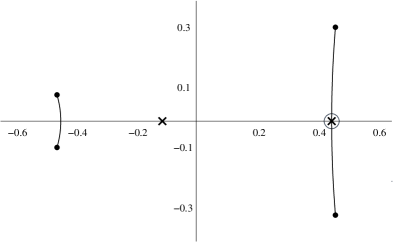
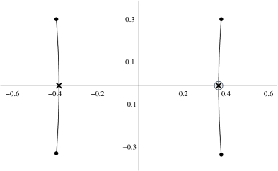
(a)	(b)
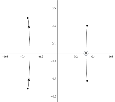
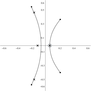
(c)	(d)
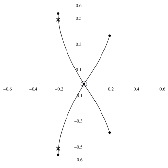
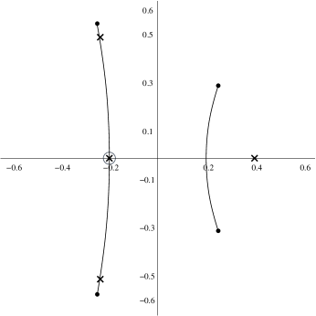
(e)	(f)

Figure 5. Drawings of the spectra of selected closed elastic rods belonging to a homotopy between a singly-covered circle and a double-covered circle, going from unknotted to a trefoil knot type along the way.

About Figure 5

This figure shows the Floquet spectra of some elastic rods (including some with special geometric features) belonging to a typical homotopy. The diagrams, which are based on Mathematica plots using equation (42), show the continuous spectrum, including the real axis, the simple points (which appear as dots), the multiple points (which are usually double points, and appear as x’s), and the Sym-Pohlmeyer reconstruction point (which is circled). In each case, the spectrum is translated in the real direction so that the sum of the branch points is zero. The stages of the homotopy shown are:

1. an unknotted rod, with branch points $-0.454\pm 0.095\mathrm{i}$ and $0.454\pm 0.324\mathrm{i}$ in the upper half plane;

2. a constant torsion rod, with symmetric spectrum and branch points $\pm 0.388\pm 0.316\mathrm{i}$ (note the coalescence, at the base of the left-hand spine, of two double points, one of which previously entered from the left);

3. another unknotted rod, with branch points $-0.342\pm 0.409846\mathrm{i}$ and $0.342\pm 0.320\mathrm{i}$, and double points migrating out along the left-hand spine;

4. a third unknotted rod, with branch points $-0.206\pm 0.545\mathrm{i}$ and $0.205\pm 0.366\mathrm{i}$, and a double point which has entered from the left;

5. an Eulerian elastic curve, with branch points $-0.201\pm 0.546\mathrm{i}$ and $0.201\pm 0.370\mathrm{i}$, and a multiple point of order six at the origin, where the zeros of the quasimomentum differential have coalesced;

6. a knotted rod, with branch points $-0.251\pm 0.557\mathrm{i}$ and $0.251\pm 0.308\mathrm{i}$, and the reconstruction point now on the left-hand spine.

As the homotopy continues, the right-hand spine shrinks toward the real axis. After the change in knot type, the spectrum does not look qualitatively different from frame (f).

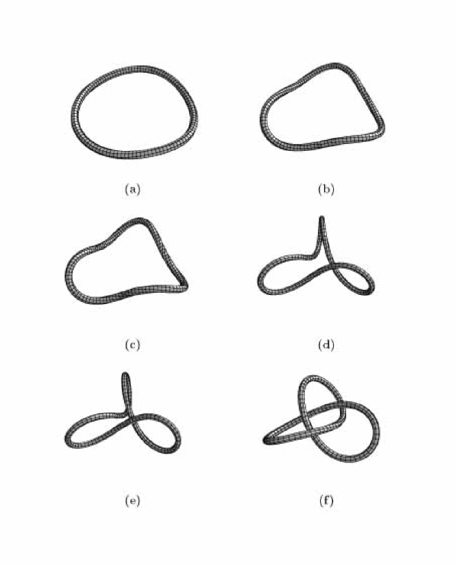
Figure 6. Drawings of the the rod centerlines corresponding to the spectra in Figure 5.

4. Symmetric Solutions

As before, let $\Sigma$ be a smooth hyperelliptic curve of genus $g$, defined by

$$\mu^{2}=\prod_{j=1}^{2g+2}(\lambda-\lambda_{j}),$$

where the branch points are symmetric about the real axis, i.e., $\lambda_{g+k}=\overline{\lambda}_{k}$ for $1\leq k\leq g+1$. In this section, we assume that the branch points are also symmetric about the origin. Then, in addition to the sheet interchange automorphism $\iota$, $\Sigma$ has an automorphism

$$\sigma:(\lambda,\mu)\mapsto(-\lambda,(-1)^{g+1}\mu),$$ (43)

the sign being chosen so that $\sigma$ fixes the points $\infty_{+}$ and $\infty_{-}$ on $\Sigma$. We shall refer to such hyperelliptic curves, and the NLS potentials that arise from them, as symmetric.

4.1. Consequences of Symmetry

In order to see how the standard homology basis behaves under automorphism $\sigma$, it is convenient to define an extra cycle $a_{g+1}$, as shown in Figure 1. Then, in terms of the $a_{j}$ for $j\leq g$ and the clockwise cycle $\ell$ about $\infty_{+}$,

$$a_{g+1}\sim-\ell-\sum_{j=1}^{g}a_{j}.$$ (44)

(Here and below, $\sim$ indicates equivalence of basepoint-free homology cycles within $\Sigma\backslash\{\infty_{+},\infty_{-}\}$.)

Proposition 4.1.

For $1\leq j\leq g$, $\sigma(a_{j})\sim a_{g+2-j}$, and

$$\sigma(b_{j})\sim\left\{\begin{aligned} a_{g+1}+a_{1}-b_{1},\qquad&j=1,\\ b_{g+2-j}+a_{1}-b_{1},\qquad&j>1.\end{aligned}\right.$$

Let the homology classes be grouped symbolically into row vectors of length $g$:

$$\underline{a}=(a_{1},\ldots,a_{g}),\qquad\underline{b}=(b_{1},\ldots,b_{g}).$$

Using this notation, and using (44) to substitute for $a_{g+1}$, we may express the results of the proposition in more compact form as

$$\sigma(\underline{a})\sim\underline{a}M-\underline{\ell},\qquad\sigma(\underline{b})\sim\underline{b}\,{}^{t}\negthinspace{M}+\underline{a}(M-{}^{t}\negthinspace{M})-\underline{\ell},$$

where $\underline{\ell}$ is the row vector $(\ell,0,\ldots,0)$, and

$$M=\begin{bmatrix}-1&0&0&\ldots&0&0\\ -1&0&0&\ldots&0&1\\ -1&0&0&\ldots&1&0\\ {6}\\ -1&0&1&\ldots&0&0\\ -1&1&0&\ldots&0&0\end{bmatrix}_{g\times g}.$$

(In particular, $M=\begin{bmatrix}-1&0\\ -1&1\end{bmatrix}$ when $g=2$.)

Remark 4.2.

It is also convenient to group the holomorphic differentials of $\Sigma$ into column vectors. For example, if the ‘coordinate differentials’ $\nu_{j}=(\lambda^{g-j}/\mu)\mathrm{d}\lambda$, which are holomorphic for $1\leq j\leq g$, are grouped into a column vector $\nu$, then the vector of normalized holomorphic differentials is given by

$$\omega=2\pi\mathrm{i}\underline{A}^{-1}\nu,$$

where $\underline{A}=\nu\cdot\underline{a}$ is the $g\times g$ matrix of period integrals of the coordinate differentials, and we represent integration of a differential over a cycle by a dot. Then the Riemann matrix $\mathcal{B}$ is given by

$$\mathcal{B}=2\pi\mathrm{i}\underline{A}^{-1}(\nu\cdot\underline{b}).$$

Using the formula (43) and the transformation of the $a$-cycles under $\sigma$, it is easy to check that the Abelian differentials transform as follows:

$$\sigma^{*}\mathrm{d}\Omega_{1}=-\mathrm{d}\Omega_{1},\quad\sigma^{*}\mathrm{d}\Omega_{2}=\mathrm{d}\Omega_{2},\quad\sigma^{*}\mathrm{d}\Omega_{3}=\mathrm{d}\Omega_{3}-\omega_{1}.$$

(For example, $\sigma^{*}\mathrm{d}\Omega_{3}$ has the same asymptotics as $\mathrm{d}\Omega_{3}$, but has period $-2\pi\mathrm{i}$ on the cycle $a_{1}$.) Integrating each of these over the $b$-cycles, we obtain

$$M\mathbf{V}=-\mathbf{V},\quad M\mathbf{W}=\mathbf{W},\quad M\mathbf{r}=\mathbf{r}+(\mathcal{B}-2\pi\mathrm{i}I)_{1},$$ (45)

where the subscript one will denote the first column in a matrix or first entry in a vector. Similarly, $\sigma^{*}\omega=M\omega$, giving

$$\mathcal{B}=M\mathcal{B}\,{}^{t}\negthinspace{M}+2\pi\mathrm{i}(I-M{}^{t}\negthinspace{M}),$$ (46)

Note that $M^{2}=I$, and $\mathbf{V},\mathbf{W}$ belong respectively to the $-1$ and $+1$-eigenspaces of $M$, which we will denote as ${\mathcal{M}}_{-}$ and ${\mathcal{M}}_{+}$. It is easy to verify that $\dim{\mathcal{M}}_{-}=\lceil g/2\rceil$ while $\dim{\mathcal{M}}_{+}=\lceil(g-1)/2\rceil$.

Since the symmetric assumption $c=\sum_{j=1}^{2g+2}\lambda_{j}=0$, then (64) from the appendix gives

$$E =-\dfrac{1}{\pi\mathrm{i}}\sum_{j=1}^{g}\int_{a_{j}}\lambda\omega_{j}=-\dfrac{1}{\pi\mathrm{i}}\operatorname{tr}\left(\lambda\omega\cdot\underline{a}\right)=-\dfrac{1}{\pi\mathrm{i}}\operatorname{tr}\left(\sigma^{*}(\lambda\omega)\cdot\sigma(\underline{a})\right)$$

$$=-\dfrac{1}{\pi\mathrm{i}}\operatorname{tr}\left(\sigma^{*}(\lambda\omega)\cdot(\underline{a}M-\underline{\ell})\right)=\dfrac{\operatorname{tr}\left(\lambda M\omega\cdot\underline{a}M\right)}{\pi\mathrm{i}}+2\operatorname{tr}\left(\sigma^{*}(\lambda\underline{A}^{-1}\nu)\cdot\underline{\ell}\right)$$

$$=\dfrac{\operatorname{tr}\left(\lambda M^{2}\omega\cdot\underline{a}\right)}{\pi\mathrm{i}}+2\sum_{j=1}^{g}(\underline{A}^{-1})_{1j}\int_{\ell}\sigma^{*}\left(\dfrac{\lambda^{g+1-j}\mathrm{d}\lambda}{\mu}\right)=-E+4\pi\mathrm{i}(\underline{A}^{-1})_{11}.$$

(In the last step, the integral has a residue about $\infty_{+}$ only when $j=1$.) Therefore, using (66)

$$E=2\pi\mathrm{i}\left(\underline{A}^{-1}\right)_{11}=\tfrac{1}{2}V_{1}.$$ (47)

4.2. Results

The following results apply only to filaments reconstructed at the origin, i.e., $\Lambda_{0}=0$ in the Sym-Pohlmeyer formula. Note that, with this choice, smooth closure of the filament is not automatic. When $g$ is even, the origin is automatically a zero of $\mathrm{d}\Omega_{1}$, but it is not automatically a double point.

Theorem 4.3.

Assume $\Sigma$ is symmetric. Let $q(s,t)$ be the NLS potential associated to $(\Sigma,\mathbf{D})$, given by (53). Let $\Lambda\subset{\mathbb{Z}}^{g}$ be the one-dimensional lattice of vectors $\mathbf{m}$ such that $m_{1}=0$ and $m_{2}=\ldots=m_{g}$ is odd. (Note that $\Lambda\subset{\mathcal{M}}_{+}$.) Suppose $t_{0}$ is such that

$$\mathbf{D}+M\mathbf{D}-2\mathrm{i}\mathbf{W}t_{0}=\pi\mathrm{i}\mathbf{m}$$ (48)

for some $\mathbf{m}\in\Lambda$. Then $q(s,t_{0})$ is the potential for a planar filament.

(Note that, following §5.2, the vector $\mathbf{D}$ may be assumed to be purely imaginary.)

Corollary 4.4.

If $\Sigma$ is symmetric and $g=2$ or $g=3$, then ${\mathcal{M}}_{+}$ is one-dimensional, and the filament is planar at regular intervals in time.

By observing that, in low genus, $\mathbf{W}$ must be a multiple of ${}^{t}\negthinspace{\,(0,1,\ldots,1)}\in{\mathcal{M}}_{+}$, we deduce that the gap between planar times is $\pi/W_{g}$. It is possible that higher-genus filaments may be planar at isolated times, but Thm. 4.3 only implies this if the projection of $\mathbf{D}$ into ${\mathcal{M}}_{+}$ lies along one of a countable number of lines parallel to $\mathbf{W}$. If that is the case, then planarity at repeated times is possible if $\mathbf{W}$ is a multiple of ${}^{t}\negthinspace{\,(0,1,\ldots,1)}$.

Proof of Theorem 4.3.

Let $\mathbf{D}^{\prime}=\mathbf{D}-\mathrm{i}\mathbf{W}t_{0}$. To prove planarity at time $t_{0}$ it suffices to prove that $q_{0}(s)$, which we define as

$$q_{0}(s):=\dfrac{q(s,t_{0})}{A\exp(\mathrm{i}Nt_{0})}=\exp(-\mathrm{i}Es)\dfrac{\theta(\mathrm{i}\mathbf{V}s+\mathbf{r}-\mathbf{D}^{\prime})}{\theta(\mathrm{i}\mathbf{V}s-\mathbf{D}^{\prime})},$$ (49)

is the potential of a planar curve, i.e., the real and imaginary parts of $q_{0}$, which are the curvatures for a natural framing along the curve, satisfy a constant-coefficient homogeneous linear equation (see, e.g., [2]). To this end, compute

$$\overline{q_{0}(s)}=\exp(+\mathrm{i}Es)\dfrac{\theta(-\mathrm{i}\mathbf{V}s+\bar{\mathbf{r}}+\mathbf{D}^{\prime})}{\theta(-\mathrm{i}\mathbf{V}s+\mathbf{D}^{\prime})}=\exp(\mathrm{i}Es)\dfrac{\theta(-\mathrm{i}\mathbf{V}s+\mathbf{r}+\mathbf{D}^{\prime})}{\theta(\mathrm{i}\mathbf{V}s-\mathbf{D}^{\prime})},$$

using the fact that $\mathbf{D}^{\prime}$ is pure imaginary, $\bar{\mathbf{r}}\equiv\mathbf{r}$ mod $2\pi\mathrm{i}$, and $\theta$ is an even function. Then, using $\mathbf{D}^{\prime}=-M\mathbf{D}^{\prime}+\pi\mathrm{i}\mathbf{m}$ and (45), we have

$$\overline{q_{0}(s)}=\exp(\mathrm{i}Es)\dfrac{\theta(M(\mathrm{i}\mathbf{V}s+\mathbf{r}+\mathcal{B}_{1}-\mathbf{D}^{\prime}+\pi\mathrm{i}\mathbf{m}))}{\theta(\mathrm{i}\mathbf{V}s-\mathbf{D}^{\prime})}.$$

The theta-function in the numerator is given by the series

$$\sum_{\mathbf{n}\in{\mathbb{Z}}^{g}}\exp\langle\mathbf{n},M(\mathrm{i}\mathbf{V}s+\mathbf{r}+\mathcal{B}_{1}-\mathbf{D}^{\prime}+\pi\mathrm{i}\mathbf{m})+\tfrac{1}{2}\mathcal{B}\mathbf{n}\rangle\\ =\sum_{\mathbf{n}}\exp\langle{}^{t}\negthinspace{M}\mathbf{n},\mathrm{i}\mathbf{V}s+\mathbf{r}+\mathcal{B}_{1}-\mathbf{D}^{\prime}+\pi\mathrm{i}\mathbf{m}+\tfrac{1}{2}M\mathcal{B}\mathbf{n}\rangle\\ =\sum_{\mathbf{n}}\exp\langle{}^{t}\negthinspace{M}\mathbf{n},\mathrm{i}\mathbf{V}s+\mathbf{r}+\mathcal{B}_{1}-\mathbf{D}^{\prime}+\pi\mathrm{i}\mathbf{m}+\tfrac{1}{2}(\mathcal{B}{}^{t}\negthinspace{M}+2\pi\mathrm{i}(M-{}^{t}\negthinspace{M}))\mathbf{n}\rangle\\ =\sum_{\mathbf{n}}\exp\langle{}^{t}\negthinspace{M}\mathbf{n},\mathrm{i}\mathbf{V}s+\mathbf{r}+\mathcal{B}_{1}-\mathbf{D}^{\prime}+\tfrac{1}{2}\mathcal{B}{}^{t}\negthinspace{M}\mathbf{n}\rangle\exp\langle{}^{t}\negthinspace{M}\mathbf{n},\pi\mathrm{i}(\mathbf{m}+(M-{}^{t}\negthinspace{M})\mathbf{n})\rangle,$$

where in the third line we use the substitution $M\mathcal{B}=\mathcal{B}{}^{t}\negthinspace{M}+2\pi\mathrm{i}(M-{}^{t}\negthinspace{M})$, derived from (46). Now we observe that the second factor in the last line is equal to one. For, let $s=n_{2}+\ldots+n_{g}$. Then

$$\langle{}^{t}\negthinspace{M}\mathbf{n},\mathbf{m}+(M-{}^{t}\negthinspace{M})\mathbf{n}\rangle=sm_{2}+s(-n_{1}-s)-n_{1}s=s(m_{2}-2n_{1}-s).$$

When $s$ is odd, the factor $(m_{2}-2n_{1}-s)$ is even, and vice-versa. Hence, because ${}^{t}\negthinspace{M}\mathbf{n}$ ranges over all points of ${\mathbb{Z}}^{g}$,

$$\theta(M(\mathrm{i}\mathbf{V}s+\mathbf{r}+\mathcal{B}_{1}-\mathbf{D}^{\prime}+\pi\mathrm{i}\mathbf{m}))=\theta(\mathrm{i}\mathbf{V}s+\mathbf{r}+\mathcal{B}_{1}-\mathbf{D}^{\prime}).$$

Next, using the quasi-periodicity of $\theta$,

$$\overline{q_{0}(s)} =\exp(\mathrm{i}Es)\dfrac{\theta(\mathrm{i}\mathbf{V}s+\mathbf{r}+\mathcal{B}_{1}-\mathbf{D}^{\prime})}{\theta(\mathrm{i}\mathbf{V}s-\mathbf{D}^{\prime})}=\exp(\mathrm{i}Es)\exp(-\mathrm{i}V_{1}s-r_{1}+D^{\prime}_{1})\dfrac{\theta(\mathrm{i}\mathbf{V}s+\mathbf{r}-\mathbf{D}^{\prime})}{\theta(\mathrm{i}\mathbf{V}s-\mathbf{D}^{\prime})}$$

$$=\exp(-\mathrm{i}Es)\exp(D^{\prime}_{1}-r_{1})\dfrac{\theta(\mathrm{i}\mathbf{V}s+\mathbf{r}-\mathbf{D}^{\prime})}{\theta(\mathrm{i}\mathbf{V}s-\mathbf{D}^{\prime})}=\exp(D^{\prime}_{1}-r_{1})q_{0}(s),$$

using the formula (47) for $E$. Since $q_{0}(s)$ is a constant multiple of its complex conjugate, it is the potential of a planar curve. ∎

Figure 7. Genus 2 symmetric filament, generated using $\mathbf{D}=0$, at times $t=(.4k-1)(\pi/2W_{2})$, for $k$ from $0$ to $5$. This illustrates the periodic planarity of Thm. 4.3, the sphericity of Remark 4.5, and persistent planes of symmetry of Thm. 4.8.

When a filament is planar at regular intervals (as predicted by Cor. 4.4), these planar forms are congruent to each other. For, if $t_{0}$ is a planar time and we increase time to $t_{1}=t_{0}+2\pi/W_{g}$, then $\mathbf{D}^{\prime}$ is decreased by an integer vector times $2\pi\mathrm{i}$. The modified potential $q_{0}$, defined in (49), is unchanged. So, $q(s,t_{1})/q(s,t_{0})$ is a unit modulus constant, and the filament at time $t_{2}$ is congruent to that at time $t_{0}$. Moreover, the isometry of ${\mathbb{R}}^{3}$ that carries the filament at time $t_{0}$ to time $t_{1}$ will be repeated in the evolution from $t_{1}$ to subsequent planar times $t_{2},t_{3}$, etc. However, computer experiments in genus two show that the curve at time $t_{1/2}=t_{0}+\pi/W_{g}$ is also congruent to the curve at time $t_{0}$, but this doesn’t happen in genus three.

Remark 4.5.

Another phenomenon (which so far is only experimentally verified) is that in genus two, between the planar times $t_{0},t_{1/2},t_{1},\ldots$, the curve lies on a sphere whose center and radius vary with time. (This can be checked numerically by evaluating the real and imaginary parts of the potential $q(s,t)$ at a fixed time, and verifying that they satisfy an inhomogeneous linear equation.) Vortex filament flow solutions obtained as Bc̈klund transformations of translating circles also lie on spheres [6].

Proposition 4.6.

Let $q(s)$ be the potential for a curve ${\boldsymbol{\gamma}}(s)$ in ${\mathbb{R}}^{3}$. If $q(-s)=q(s)$, then the curve is symmetric under reflection in the normal plane through ${\boldsymbol{\gamma}}(0)$. If $\overline{q(s)}=q(-s)$, then the curve is symmetric under a 180-degree rotation about the normal line through ${\boldsymbol{\gamma}}(0)$.

Proof.

Let $T(s),N_{1}(s),N_{2}(s)$ be an oriented natural frame along ${\boldsymbol{\gamma}}$, with natural curvatures $k_{1},k_{2}$ which are the real and imaginary parts of $q(s)$ respectively. Let $\widetilde{{\boldsymbol{\gamma}}}(s)={\boldsymbol{\gamma}}(-s)$. Then in the first case $(-T(-s),N_{1}(-s),N_{2}(-s))$ is an oppositely-oriented natural frame for $\widetilde{{\boldsymbol{\gamma}}}$ with the same curvature functions as the given oriented frame for ${\boldsymbol{\gamma}}$. Hence $\widetilde{{\boldsymbol{\gamma}}}(s)$ must be congruent to ${\boldsymbol{\gamma}}(s)$ under an orientation-reversing isometry. Since that motion must fix ${\boldsymbol{\gamma}}(0)$ and $N_{1}(0),N_{2}(0)$, then it must be reflection in the normal plane through ${\boldsymbol{\gamma}}(0)$. In the second case, $(-T(-s),N_{1}(-s),-N_{2}(-s))$ is a similarly-oriented natural frame for $\widetilde{{\boldsymbol{\gamma}}}$ with the same curvatures, and $\widetilde{{\boldsymbol{\gamma}}}(s)$ must be congruent to ${\boldsymbol{\gamma}}(s)$ under an orientation-preserving isometry that fixes ${\boldsymbol{\gamma}}(0)$ and the line through ${\boldsymbol{\gamma}}(0)$ along $N_{1}(0)$. (Since $k_{2}(0)=0$, this is the normal line at ${\boldsymbol{\gamma}}(0)$.) ∎

Proposition 4.7.

Let $\Sigma$ be symmetric, and assume there are $s_{0}$ and $t_{0}$ such that

$$\mathbf{D}-(\mathrm{i}\mathbf{V}s_{0}+\mathrm{i}\mathbf{W}t_{0})=\pi\mathrm{i}\mathbf{k}$$ (50)

for some vector $\mathbf{k}$ of odd integers. Then the filament is symmetric under a 180-degree rotation about the normal line through ${\boldsymbol{\gamma}}(s_{0},t_{0})$

Proof.

Let $s^{\prime}=s-s_{0}$, and let

$$q_{0}(s^{\prime})=\dfrac{q(s,t_{0})}{A\exp(-\mathrm{i}Es_{0}+\mathrm{i}Nt_{0})}=\exp(-\mathrm{i}Es^{\prime})\dfrac{\theta(\mathrm{i}\mathbf{V}s^{\prime}+\mathbf{r}-\pi\mathrm{i}\mathbf{k})}{\theta(\mathrm{i}\mathbf{V}s^{\prime}-\pi\mathrm{i}\mathbf{k})}$$

It is easy to see that

$$\overline{q_{0}(s^{\prime})}=\exp(+\mathrm{i}Es^{\prime})\dfrac{\theta(-\mathrm{i}\mathbf{V}s^{\prime}+\bar{\mathbf{r}}+\pi\mathrm{i}\mathbf{k})}{\theta(-\mathrm{i}\mathbf{V}s^{\prime}+\pi\mathrm{i}\mathbf{k})}=\exp(\mathrm{i}Es^{\prime})\dfrac{\theta(-\mathrm{i}\mathbf{V}s^{\prime}+\mathbf{r}-\pi\mathrm{i}\mathbf{k})}{\theta(-\mathrm{i}\mathbf{V}s^{\prime}-\pi\mathrm{i}\mathbf{k})}=q_{0}(-s^{\prime}),$$

using the $2\pi\mathrm{i}$-periodicity of $\theta$. Since $|A|q_{0}(s^{\prime})$ is a potential for the filament ${\boldsymbol{\gamma}}(s,t_{0})$, then the result follows by Prop. 4.6. ∎

Theorem 4.8.

Assume $\Sigma$ is symmetric and of genus 2. Then there is a fixed plane in ${\mathbb{R}}^{3}$ such that at each time the filament is symmetric under reflection in that plane. At each ‘planar time’ $t_{0}$ given by Thm. 4.3, the plane containing the filament is perpendicular to the plane fixed by the reflection.

Proof.

Let $t_{0}$ be a planar time, i.e., suppose (48) is true for some $\mathbf{m}\in\Lambda$. Then there exist $s_{0}$ and an odd integer vector $\mathbf{k}$ such that (50) is satisfied. For, (48) says that the projection of $\mathbf{D}^{\prime}=\mathbf{D}-\mathrm{i}\mathbf{W}t_{0}$ into ${\mathcal{M}}_{+}$ is $\tfrac{1}{2}\mathbf{m}$. Given this, then (50) implies that $\mathbf{k}+M\mathbf{k}=\mathbf{m}$, which amounts to $2k_{2}-k_{1}=m_{2}$. Given any $\mathbf{k}$ that satisfies this condition, there exists an $s_{0}$ that satisfies (50), because $\mathbf{V}$ spans ${\mathcal{M}}_{-}$.

Thus, the curve is symmetric under rotation $\mathcal{T}$ about an axis $L$ through ${\boldsymbol{\gamma}}(s_{0},t_{0})$. However, since the filament is also planar at time $t_{0}$, the rotation $\mathcal{T}$ can be replaced by the reflection $\mathcal{R}$ in the plane through $L$ perpendicular to the plane containing the filament.

To complete the proof, we use the symmetry properties of the vortex filament flow

$${\boldsymbol{\gamma}}_{t}={\boldsymbol{\gamma}}_{s}\times{\boldsymbol{\gamma}}_{ss}.$$

If ${\boldsymbol{\gamma}}(s,t)$ is a solution, and $\mathcal{T}$ is a orientation-preserving isometry of ${\mathbb{R}}^{3}$, then it is easy to check that $\widetilde{{\boldsymbol{\gamma}}}(s,t):=\mathcal{T}({\boldsymbol{\gamma}}(s,t))$ is another solution. In particular, if $\widetilde{{\boldsymbol{\gamma}}}(s,t_{0})={\boldsymbol{\gamma}}(s-c,t_{0})$ for some $c$ and some time $t_{0}$, then this equation holds at all times. In other words, symmetry under $\mathcal{T}$ is preserved by the flow.

Similarly, if $\mathcal{R}$ is an orientation-reversing isometry, then $\widetilde{{\boldsymbol{\gamma}}}(s,t):=\mathcal{R}({\boldsymbol{\gamma}}(-s,t))$ is another solution. Since ${\boldsymbol{\gamma}}$ is symmetric under reflection $\mathcal{R}$ at time $t_{0}$, and this symmetry reverses orientation along ${\boldsymbol{\gamma}}$, then $\mathcal{R}({\boldsymbol{\gamma}}(-s,t))={\boldsymbol{\gamma}}(s-c,t_{0})$ for some $c$, and it follows that this relationship persists in time. ∎

Figure 8. Genus 3 symmetric filament, generated using $\mathbf{D}=0$, at times $t=(.4k-1)(\pi/2W_{2})$, for $k$ from $0$ to $5$.. Note the persistent self-intersections in the plane of reflection symmetry. The curve returns to its original shape, in a rotated plane.

Remark 4.9.

At a planar time, a filament must cross the axis of symmetry at least once, since the filament is connected to its reflection. If it crosses the axis in a direction that is not perpendicular to the axis, a self-intersection occurs at this point. The fact that reflection symmetry persists as the curve lifts out of the plane implies that these self-intersections also persist (see Figures 7 and 8). However, it is possible that, as the curve evolves, two self-intersections may coalesce and disappear, while maintaining reflection symmetry.

Note that not all planar curves that are symmetric about an axis have self-intersections which are preserved by the flow. It is easy to draw examples where the reflection symmetry preserves the orientation along the curve (rather than reversing it, which is the property used in the proof of Theorem 4.8). Then, under the filament flow, the strands immediately pull away in opposite directions from the self-intersections. In this case, the symmetry is the restriction of an orientation-preserving 180-degree rotation in ${\mathbb{R}}^{3}$, and such rotational symmetry persists as the filament evolves.

Remark 4.10.

The argument in the proof of Theorem 2 relies on the fact that, when $g=2$, $\mathbf{V}$ and $\mathbf{W}$ span ${\mathbb{R}}^{g}$. However, given a symmetric hyperelliptic curve of genus $g\geq 3$, there are plenty of potentials to which the argument in the proof of Theorem 4.8 applies (see Figure 8). For, given any vector $\mathbf{k}$ of odd integers, we may choose an imaginary vector $\mathbf{D}$ so that (50) is satisfied for some $s_{0}$ and $t_{0}$. Then $\mathbf{D}$ also satisfies (48) if and only if the differences $k_{g-j}-k_{2+j}$, $j\geq 0$, are all equal. The latter condition is vacuous when $g=3$. Thus, in genus 3 the set of appropriate divisors corresponds to the image of the affine lattice of odd integer vectors in the quotient vector space ${\mathbb{R}}^{3}/\{\mathbf{V},\mathbf{W}\}$. (Changing $\mathbf{D}$ by a multiple of $\mathbf{V}$ or $\mathbf{W}$ merely corresponds to a shift in $s_{0}$ or $t_{0}$.)

‘

5. Appendix

In this appendix, we will indicate how the formulas for finite-gap NLS Baker-Akhiezer functions developed in §2 are related to those given in the monograph by Belokolos, Bobenko, Enol’skii, Its and Matveev [1]. We will also develop (from a slightly different perspective than [1]) the reality condition which must be satisfied by the divisor, and discuss how to compute some of the quantities used in the expression for the finite-gap NLS potential.

5.1. Alternative Eigenfunction Formulas

From §2.1, we had

$$\psi^{1}(P;s,t)=\dfrac{g_{+}(P)}{g_{+}(\infty_{-})}\exp\left(\mathrm{i}s(\Omega_{1}(P)-\tfrac{E}{2})+\mathrm{i}t(\Omega_{2}(P)+\tfrac{N}{2})\right)\\ \times\dfrac{\theta(\boldsymbol{\mathcal{A}}(P)+\mathrm{i}\mathbf{V}s+\mathrm{i}\mathbf{W}t-\boldsymbol{\mathcal{A}}(\mathcal{D}_{+})-\boldsymbol{\mathcal{K}})\,\theta(\boldsymbol{\mathcal{A}}(\infty_{-})-\boldsymbol{\mathcal{A}}(\mathcal{D}_{+})-\boldsymbol{\mathcal{K}})}{\theta(\boldsymbol{\mathcal{A}}(\infty_{-})+\mathrm{i}\mathbf{V}s+\mathrm{i}\mathbf{W}t-\boldsymbol{\mathcal{A}}(\mathcal{D}_{+})-\boldsymbol{\mathcal{K}})\,\theta(\boldsymbol{\mathcal{A}}(P)-\boldsymbol{\mathcal{A}}(\mathcal{D}_{+})-\boldsymbol{\mathcal{K}})}$$

and

$$\psi^{2}(P;s,t)=\dfrac{g_{-}(P)}{g_{-}(\infty_{+})}\exp\left(\mathrm{i}s(\Omega_{1}(P)+\tfrac{E}{2})+\mathrm{i}t(\Omega_{2}(P)-\tfrac{N}{2})\right)\\ \times\dfrac{\theta(\boldsymbol{\mathcal{A}}(P)+\mathrm{i}\mathbf{V}s+\mathrm{i}\mathbf{W}t-\boldsymbol{\mathcal{A}}(\mathcal{D}_{-})-\boldsymbol{\mathcal{K}})\,\theta(\boldsymbol{\mathcal{A}}(\infty_{+})-\boldsymbol{\mathcal{A}}(\mathcal{D}_{-})-\boldsymbol{\mathcal{K}})}{\theta(\boldsymbol{\mathcal{A}}(\infty_{+})+\mathrm{i}\mathbf{V}s+\mathrm{i}\mathbf{W}t-\boldsymbol{\mathcal{A}}(\mathcal{D}_{-})-\boldsymbol{\mathcal{K}})\,\theta(\boldsymbol{\mathcal{A}}(P)-\boldsymbol{\mathcal{A}}(\mathcal{D}_{-})-\boldsymbol{\mathcal{K}})}.$$

Recall that $\mathrm{d}\Omega_{3}$ is the Abelian differential on $\Sigma$, with zero $a$-periods, such that

$$\mathrm{d}\Omega_{3}\sim\pm\dfrac{\mathrm{d}\lambda}{\lambda}\qquad\text{as}\ \lambda\to\infty_{\pm}.$$

Then $\oint_{\ell}\mathrm{d}\Omega_{3}=2\pi\mathrm{i}$, where $\ell$ is the clockwise cycle around $\infty_{+}$ shown in Figure 1.

Lemma 5.1.

$\oint_{b_{j}}\mathrm{d}\Omega_{3}=-r_{j}$, where $r_{j}$ denotes the $j$th entry of vector $\mathbf{r}$.

This will be proved at the end of §5.3. For now, we note that the corresponding Abelian integral $\Omega_{3}$ behaves like $\pm\log(\lambda)$ near $\infty_{\pm}$. Furthermore, we observe that the quotient

$$f(P)=\exp(\Omega_{3}(P))\dfrac{\theta(\boldsymbol{\mathcal{A}}(P)-\mathbf{D}-\mathbf{r})}{\theta(\boldsymbol{\mathcal{A}}(P)-\mathbf{D})}$$

is a well-defined meromorphic function on $\Sigma$. For, if the paths of integration in the integrals $\Omega_{3}(P)$ and $\boldsymbol{\mathcal{A}}(P)$ are changed by the addition of the same $a$-cycle, each factor in $f(P)$ is unchanged; if the cycle $b_{j}$ is added, then $f(P)$ is modified by the factor

$$\exp\left(\oint_{b_{j}}\mathrm{d}\Omega_{3}\right)\exp(r_{j})=1.$$

Note that if, say, we confine the path of integration for $\Omega_{3}$ to the interior of the cut Riemann surface $\Sigma_{0}$ described in §2.1, then $\exp(\Omega_{3}(P))$ has a pole at $\infty_{+}$ and a zero at $\infty_{-}$. Consequently, $f(P)$ has pole divisor $\mathcal{D}_{+}+\infty_{+}$ and zero divisor $\mathcal{D}_{-}+\infty_{-}$. It follows that

$$\exp(\Omega_{3}(P))\dfrac{\theta(\boldsymbol{\mathcal{A}}(P)-\mathbf{D}-\mathbf{r})}{\theta(\boldsymbol{\mathcal{A}}(P)-\mathbf{D})}\times\dfrac{g_{+}(P)}{g_{-}(P)}$$ (51)

is a nonzero constant.

We can express this constant in terms of the asymptotic behavior of $\Omega_{3}$ and $g_{+}$. Namely, suppose $P$ is near $\infty_{+}$ and lies over the real axis in the $\lambda$-plane. Let $C_{P}$ be a path from $P$ to $\iota(P)$ in the interior of $\Sigma_{0}$, such that $C_{P}$ is invariant under sheet interchange. Let $a_{g+1}$ be the cycle around the rightmost branch cut, which satisfies the homological equivalence (44) within $\Sigma-\{\infty_{+},\infty_{-}\}$. Then we have

$$\int_{C_{P}}\overline{\mathrm{d}\Omega_{3}}=\int_{\tau(C_{P})}\mathrm{d}\Omega_{3}=\int_{C_{P}+a_{g+1}}\mathrm{d}\Omega_{3}=-2\pi\mathrm{i}+\int_{C_{P}}\mathrm{d}\Omega_{3},$$

where $\tau:(\lambda,\mu)\mapsto(\overline{\lambda},\overline{\mu})$ is complex conjugation on $\Sigma$. Therefore,

$$\lim_{P\to\infty_{+}}\left(\int_{C_{P}}\mathrm{d}\Omega_{3}-2\log\lambda(P)\right)=\pi\mathrm{i}-\log\beta$$ (52)

for some positive real number $\beta$. (In terms of the notation in [1], the above limit is written as $-\log\omega_{0}$ for a negative real number $\omega_{0}$.) Therefore,

$$\exp(\Omega_{3}(P))\sim\dfrac{\mathrm{i}}{\sqrt{\beta}}\lambda\qquad\text{as}\ P\to\infty_{+}.$$

Suppose that $g_{+}(P)=\dfrac{1}{\alpha\lambda}+O(\lambda^{-2})$ when $P$ is near $\infty_{+}$, for some constant $\alpha$. Then letting $P$ tend to $\infty_{+}$ in (51) gives

$$\exp(\Omega_{3}(P))\dfrac{\theta(\boldsymbol{\mathcal{A}}(P)-\mathbf{D}-\mathbf{r})}{\theta(\boldsymbol{\mathcal{A}}(P)-\mathbf{D})}\times\dfrac{g_{+}(P)}{g_{-}(P)}=\dfrac{\mathrm{i}}{\alpha\sqrt{\beta}}\dfrac{\theta(\mathbf{D})}{\theta(\mathbf{D}-\mathbf{r})}.$$

Solving this equation for $g_{-}(P)$ and substituting in $\psi^{2}$ gives

$$\psi^{2}=g_{+}(P)\dfrac{\alpha\sqrt{\beta}}{\mathrm{i}}\exp\left(\mathrm{i}s(\Omega_{1}(P)+\tfrac{E}{2})+\mathrm{i}t(\Omega_{2}(P)-\tfrac{N}{2})+\Omega_{3}(P)\right)\\ \times\dfrac{\theta(\boldsymbol{\mathcal{A}}(P)+\mathrm{i}\mathbf{V}s+\mathrm{i}\mathbf{W}t-\mathbf{D}-\mathbf{r})\,\theta(\mathbf{D}-\mathbf{r})}{\theta(\mathrm{i}\mathbf{V}s+\mathrm{i}\mathbf{W}t-\mathbf{D})\,\theta(\boldsymbol{\mathcal{A}}(P)-\mathbf{D})},$$

which agrees with the formula 4.1.16 for $\psi^{2}$ in [1], up to the multiplicative factor of $g_{+}(P)$. Similarly, $\psi^{1}$ coincides with the formula for $\psi^{1}$ in [1] except for multiplication by $g_{+}(P)$. Since our vector-valued function and that of [1] differ only by multiplication by a scalar that is independent of $s$ and $t$, both satisfy the NLS linear system for the same potential $q(s,t)$.

5.2. Reality Conditions

By inserting the matrix $\Psi$ defined by (17) into the NLS linear system, and expanding near $\infty_{-}$ in powers of $\lambda$, we obtain

$$q(s,t)=A\exp(-\mathrm{i}Es+\mathrm{i}Nt)\dfrac{\theta(\mathrm{i}\mathbf{V}s+\mathrm{i}\mathbf{W}t-\mathbf{D}+\mathbf{r})}{\theta(\mathrm{i}\mathbf{V}s+\mathrm{i}\mathbf{W}t-\mathbf{D})}\qquad\text{where}\ A=\dfrac{2\theta(\mathbf{D})}{\alpha\theta(\mathbf{D}-\mathbf{r})},$$ (53)

and

$$\overline{q(s,t)}=\dfrac{4\beta}{A}\exp(\mathrm{i}Es-\mathrm{i}Nt)\dfrac{\theta(\mathrm{i}\mathbf{V}s+\mathrm{i}\mathbf{W}t-\mathbf{D}-\mathbf{r})}{\theta(\mathrm{i}\mathbf{V}s+\mathrm{i}\mathbf{W}t-\mathbf{D})}.$$ (54)

It is not immediate that the second expression is the complex conjugate of the first; in fact, the reality conditions on $\mathbf{D}$ come from imposing this condition. Before computing this, we need to calculate the imaginary parts of the members of (53). Since $\tau^{*}\mathrm{d}\Omega_{j}=\overline{\mathrm{d}\Omega_{j}}$ and

$$\tau(b_{k})\sim b_{k}+\ell+\sum_{l\neq k}a_{l}$$

within $\Sigma-\{\infty_{+},\infty_{-}\}$, then $\mathbf{V}$ and $\mathbf{W}$, being the $b$-periods of $\mathrm{d}\Omega_{1}$ and $\mathrm{d}\Omega_{2}$, are real vectors. Similarly, Lemma 5.1 implies that

$$r_{k}=\overline{r_{k}}+2\pi\mathrm{i}.$$

Moreover, since $\tau^{*}\omega_{k}=\overline{\omega_{k}}$, then the Riemann matrix $\mathcal{B}$, defined by (9) satisfies

$$\overline{\mathcal{B}_{kl}}=\left\{\begin{aligned} \mathcal{B}_{kl}&\text{ for}\ k=l\\ \mathcal{B}_{kl}+2\pi\mathrm{i}&\text{ for}\ k\neq l.\end{aligned}\right.$$ (55)

It follows that $\overline{\theta(z)}=\theta(\overline{z}).$

Now comparing (53) and (54) gives the reality condition

$$\overline{A}\dfrac{\theta(-\mathrm{i}\mathbf{V}s-\mathrm{i}\mathbf{W}t-\overline{\mathbf{D}}+\overline{\mathbf{r}})}{\theta(-\mathrm{i}\mathbf{V}s-\mathrm{i}\mathbf{W}t-\overline{\mathbf{D}}}=\dfrac{4\beta}{A}\dfrac{\theta(\mathrm{i}\mathbf{V}s+\mathrm{i}\mathbf{W}t-\mathbf{D}-\mathbf{r})}{\theta(\mathrm{i}\mathbf{V}s+\mathrm{i}\mathbf{W}t-\mathbf{D})}.$$

Since poles and zeros must match up, we must have

$$\mathbf{D}+\overline{\mathbf{D}}=2\pi\mathrm{i}{\mathbf{n}}+\mathcal{B}{\mathbf{m}},$$ (56)

where $\mathbf{m},\mathbf{n}\in{\mathbb{Z}}^{g}$ are such that

$$|A|^{2}\exp(\langle\mathbf{m},\mathbf{r}\rangle)=4\beta.$$ (57)

Taking the imaginary part of (56), with (55) taken into account, gives

$$2n_{j}=\sum_{k\neq j}m_{k}.$$ (58)

(In particular, $\mathbf{n}=0$ when $g=1$.) Thus, all the entries of $\mathbf{m}$ have the same parity, even or odd. When $g$ is even, summing (58) over $j$ shows that $\mathbf{m}$ must be all even. If $g$ is odd and $\mathbf{m}$ is all odd, the fact that ${\sf Im}(r_{j})=\pi$ would imply that the left-hand side of (57) is negative. Thus, we can assume that $\mathbf{m}$ is all even. In this case, one can let $\mathbf{D}^{\prime}=\mathbf{D}-\tfrac{1}{2}\mathcal{B}\mathbf{m}$; then $\mathbf{D}^{\prime}$ is purely imaginary, and (53),(57) are still valid with $\mathbf{D}$ replaced by $\mathbf{D}^{\prime}$ and $\mathbf{m}$ replaced by zero. We now do this, and then our reality condition amounts to the vector $\mathbf{D}$ being purely imaginary:

$$\overline{\mathbf{D}}=-\mathbf{D}.$$ (59)

We can, without loss of generality, assume that $A$ is real and positive; then (57) gives $A=2\sqrt{\beta}$. From (53) we then get $\alpha\sqrt{\beta}=2\theta(\mathbf{D})/\theta(\mathbf{D}-\mathbf{r})$. So, omitting the common scalar multiples $g_{+}(P)\theta(\mathbf{D})/\theta(\boldsymbol{\mathcal{A}}(P)-\mathbf{D})$ from the eigenfunctions gives the simplified formulas

$$\psi^{1} =\exp\left(\mathrm{i}s(\Omega_{1}(P)-\tfrac{E}{2})+\mathrm{i}t(\Omega_{2}(P)+\tfrac{N}{2})\right)\dfrac{\theta(\boldsymbol{\mathcal{A}}(P)+\mathrm{i}\mathbf{V}s+\mathrm{i}\mathbf{W}t-\mathbf{D})}{\theta(\mathrm{i}\mathbf{V}s+\mathrm{i}\mathbf{W}t-\mathbf{D})},$$

$$\psi^{2} =-\mathrm{i}\exp\left(\mathrm{i}s(\Omega_{1}(P)+\tfrac{E}{2})+\mathrm{i}t(\Omega_{2}(P)-\tfrac{N}{2})\right)\dfrac{\theta(\boldsymbol{\mathcal{A}}(P)+\mathrm{i}\mathbf{V}s+\mathrm{i}\mathbf{W}t-\mathbf{D}-\mathbf{r})}{\theta(\mathrm{i}\mathbf{V}s+\mathrm{i}\mathbf{W}t-\mathbf{D})}.$$

We will now interpret the reality condition (59) in terms of the divisors $\mathcal{D},\mathcal{D}_{+},\mathcal{D}_{-}$ on $\Sigma$.

Proposition 5.2.

If $\overline{\mathbf{D}}=-\mathbf{D}$, then $\mathcal{D}_{-}=\iota\tau(\mathcal{D}_{+})$.

(Recall that $\iota$ denotes the sheet interchange automorphism and $\tau$ denotes complex conjugation on $\Sigma$.)

Proof.

The function $f(P)=\theta(\boldsymbol{\mathcal{A}}(P)-\mathbf{D})$ has zero divisor $\mathcal{D}_{+}$. (To make $f$ well-defined, we restrict to the cut Riemann surface $\Sigma_{0}$, assuming that the homology basis avoids the points of $\mathcal{D}_{+}$ and $\mathcal{D}_{-}$.) Therefore, the function

$$\overline{f(\iota\tau(P))}=\theta\left(\overline{\boldsymbol{\mathcal{A}}(\iota\tau(P))}+\mathbf{D}\right)$$

has zero divisor $\iota\tau(\mathcal{D}_{+})$. But since $\infty_{+}=\iota\tau(\infty_{-})$ and $(\iota\tau)^{*}\omega_{j}=-\overline{\omega_{j}}$, then

$$\boldsymbol{\mathcal{A}}(\iota\tau(P))=\int_{\infty_{-}}^{\infty_{+}}\omega+\int_{\iota\tau(\infty_{-})}^{\iota\tau(P)}\omega\\ =\mathbf{r}-\overline{\boldsymbol{\mathcal{A}}(P)}.$$

Using the fact that $\overline{r_{j}}\equiv r_{j}$ modulo $2\pi\mathrm{i}$,

$$\theta\left(\overline{\boldsymbol{\mathcal{A}}(\iota\tau(P))}+\mathbf{D}\right)=\theta(\overline{\mathbf{r}}-\boldsymbol{\mathcal{A}}(P)+\mathbf{D})=\theta(\boldsymbol{\mathcal{A}}(P)-\mathbf{D}-\mathbf{r})=\theta(\boldsymbol{\mathcal{A}}(P)-\boldsymbol{\mathcal{A}}(\mathcal{D}_{-})-\boldsymbol{\mathcal{K}}),$$

which has $\mathcal{D}_{-}$ as its zero divisor. ∎

Proposition 5.3.

Assuming $\mathcal{D}$ satisfies the Genericity Condition of §2, then $\mathcal{D}_{-}=\iota\tau(\mathcal{D}_{+})$ if and only if $\iota\tau(\mathcal{D})\sim\mathcal{D}$, where $\sim$ denotes linearly equivalence of divisors.

Before proving the lemma, we recall some pertinent facts about divisors on a Riemann surface (see, e.g., [12] or [23]). For any divisor $\mathcal{D}$, the meromorphic functions $f$ such that $\mathcal{D}+(f)\geq 0$ form a vector space $\mathcal{L}(\mathcal{D})$ with dimension $l(\mathcal{D})$. For example, a positive divisor always has $l(\mathcal{D})\geq 1$, because of the constant functions. If two divisors $\mathcal{D},\mathcal{D}^{\prime}$ are linearly equivalent, then $l(\mathcal{D})=l(\mathcal{D}^{\prime})$.

The Genericity Condition can be stated as

$$l(\mathcal{D}-\infty_{-}-\infty_{+})=0.$$ (60)

This implies that $l(\mathcal{D}_{+})=l(\mathcal{D}-\infty_{+})=1$, and similarly for $\mathcal{D}_{-}$ and $\mathcal{D}-\infty_{-}$. For, if $l(\mathcal{D}-\infty_{+})>1$, let $f_{1},f_{2}\in\mathcal{L}(\mathcal{D}-\infty_{+})$ be linearly independent; then there exists a nontrivial linear combination $c_{1}f_{1}+c_{2}f_{2}$ that vanishes at $\infty_{-}$, and this contradicts (60).

Proof of Prop. 5.3.

Suppose that $\mathcal{D}_{-}=\iota\tau(\mathcal{D}_{+})$. By construction,

$$\mathcal{D}_{+}=\mathcal{D}-\infty_{+}+(f)$$

for some meromorphic function $f$. Appying $\iota\tau$ to both sides gives

$$\mathcal{D}_{-}=\iota\tau(\mathcal{D})-\infty_{-}+\left(\overline{f\circ\iota\tau}\right).$$

Since $\mathcal{D}_{-}\sim\mathcal{D}-\infty_{-}$, then $\mathcal{D}\sim\iota\tau(\mathcal{D})$.

The same computation, run backwards, shows that if $\mathcal{D}\sim\iota\tau(\mathcal{D})$ then $\mathcal{D}_{-}\sim\iota\tau(\mathcal{D}_{+})$, i.e.,

$$\mathcal{D}_{-}+(f)=\iota\tau(\mathcal{D}_{+})$$

for some meromorphic function $f$. However, $l(\mathcal{D}_{-})=1$ implies that $\mathcal{D}_{-}+(f)\geq 0$ only when $f$ is a constant. Thus, $\mathcal{D}_{-}=\iota\tau(\mathcal{D}_{+})$. ∎

5.3. Computing $E$, $N$, $\mathbf{r}$ and $\beta$

Suppose functions $\Omega,\Omega^{\prime}$ are holomorphic on the cut Riemann surface $\Sigma_{0}$. Then by Stokes’ Theorem,

$$0=\int_{\Sigma_{0}}\mathrm{d}(\Omega^{\prime}\mathrm{d}\Omega)=\oint_{\partial\Sigma_{0}}\Omega^{\prime}\mathrm{d}\Omega=\sum_{j=1}^{g}A^{\prime}_{j}B_{j}-B^{\prime}_{j}A_{j},$$ (61)

where $A_{j}=\oint_{a_{j}}\Omega$, $B_{j}=\oint_{b_{j}}\Omega$, and similarly for the primes. (See, for example, [12].) We will use this relationship to derive formulas for $E$ and $N$ and to prove Lemma 5.1. (Our formula for $E$ is equivalent to one given without proof in [1].) The differentials we use will actually have singularities at $\infty_{\pm}$, so the left-hand side of (61) will be modified by adding the integrals of $\Omega^{\prime}\mathrm{d}\Omega$ along clockwise cycles about these points:

$$0=\sum_{j=1}^{g}A^{\prime}_{j}B_{j}-B^{\prime}_{j}A_{j}+\oint_{\ell+\iota(\ell)}\Omega^{\prime}\mathrm{d}\Omega.$$ (62)

Each of these extra terms will be $-2\pi\mathrm{i}$ times the residue of the differential at the singularity.

First, let $\Omega^{\prime}=\Omega_{1}$ and $\mathrm{d}\Omega=(\lambda^{g}/\mu)\mathrm{d}\lambda$. By expanding $\mu^{2}$ in terms of $\lambda$ and applying the binomial series, we get that, near $\infty_{\pm}$,

$$\dfrac{\mu}{\lambda^{g+1}}=\pm\left(1-\frac{c}{2}\lambda^{-1}-d\lambda^{-2}+O(\lambda^{-3})\right),$$

where $c=\sum_{j=1}^{2g+2}\lambda_{j}$ and

$$d=-\frac{1}{8}\left(c^{2}-2\sum_{j=1}^{2g+2}\lambda_{j}^{2}\right)$$ (63)

This, together with

$$\Omega_{1}=\pm(\lambda+\frac{E}{2}+o(1))$$

allows us to expand the integrand near $\infty_{\pm}$:

$$\Omega^{\prime}\mathrm{d}\Omega=-\lambda^{2}\left(1-\left(\dfrac{E-c}{2}\right)\lambda^{-1}+O(\lambda^{-2})\right)\mathrm{d}(\lambda^{-1}).$$

Since $\mathrm{d}\Omega^{\prime}=\mathrm{d}\Omega_{1}$ has no $a$-periods, from (62) we have

$$0=-2\pi\mathrm{i}(E-c)-\sum_{j=1}^{g}V_{j}\oint_{a_{j}}\dfrac{\lambda^{g}}{\mu}\mathrm{d}\lambda.$$

Thus,

$$E=c-\dfrac{1}{2\pi\mathrm{i}}\sum_{j=1}^{g}V_{j}\oint_{a_{j}}\dfrac{\lambda^{g}}{\mu}\mathrm{d}\lambda.$$ (64)

Next, let $\Omega^{\prime}=\Omega_{2}$ instead. Then

$$\Omega^{\prime}\mathrm{d}\Omega=-\lambda^{3}\left(2+c\lambda^{-1}+\left(\dfrac{N}{2}+2d+\dfrac{c^{2}}{2}\right)+O(\lambda^{-3})\right)\mathrm{d}(\lambda^{-1})$$

near $\infty_{\pm}$, and (62) gives

$$0=-2\pi\mathrm{i}\left(N+4d+c^{2}\right)-\sum_{j=1}^{g}W_{j}\oint_{a_{j}}\dfrac{\lambda^{g}}{\mu}\mathrm{d}\lambda,$$

so that

$$N=-4d-c^{2}-\dfrac{1}{2\pi\mathrm{i}}\sum_{j=1}^{g}W_{j}\oint_{a_{j}}\dfrac{\lambda^{g}}{\mu}\mathrm{d}\lambda.$$ (65)

We note that, by letting $\mathrm{d}\Omega=\omega_{j}$ and $\Omega^{\prime}=\Omega_{1}$ or $\Omega_{2}$, similar calculations give

$$0=2c_{j1}-V_{j},\qquad 0=4c_{j2}+2c\,c_{j1}-W_{j},$$ (66)

where $c_{jk}$ are the constants such that

$$\omega_{j}=\sum_{k=1}^{g}c_{jk}\dfrac{\lambda^{g-k}}{\mu}\mathrm{d}\lambda.$$

Thus, computing just the $a$-periods of the coordinate differentials $\nu_{k}=\dfrac{\lambda^{g-k}}{\mu}\mathrm{d}\lambda$ for $0\leq k\leq g$, we can determine $E,N$ and the $b$-periods of $\mathrm{d}\Omega_{1},\mathrm{d}\Omega_{2}$ algebraically.

In most experiments we have carried out, it is straightforward to calculate the $a$-periods of the coordinate differentials by numerical integration. Numerical techniques are also practical for calculating $\beta$ in the limit (52). For this purpose, we can rewrite that limit as

$$2\pi\mathrm{i}-\log\beta=2\log(\lambda_{2g+2})+2\lim_{P\to\infty_{+}}\int_{\Gamma_{P}}\left(\mathrm{d}\Omega_{3}-\lambda^{-1}\mathrm{d}\lambda\right),$$

where $\Gamma_{P}$ is the portion of $C_{P}$ from $\lambda_{2g+2}$ to $P$ on the upper sheet. Now the improper integral converges.

Proof of Lemma 5.1.

If we let $\Omega^{\prime}=\Omega_{3}$ and $\mathrm{d}\Omega=\omega_{j}$, we must make additional cuts. Let $\Sigma^{\prime}_{0}$ be the cut Riemann surface $\Sigma_{0}$ (shown in Figure 2) with an additional cut from $\infty_{-}$ to $\infty_{+}$, along $\Pi\cup\iota(\Pi)$. Then $\Omega_{3}$ is well-defined and holomorphic on $\Sigma^{\prime}_{0}$, with its values of $\Omega_{3}$ differing by $2\pi\mathrm{i}$ on each side of this cut. From (61) we obtain

$$0=-2\pi\mathrm{i}\oint_{b_{j}}\mathrm{d}\Omega_{3}-2\pi\mathrm{i}\int_{\infty_{-}}^{\infty_{+}}\omega_{j}.$$

∎

References

- [1] Belokolos E., Bobenko A.,Enolskii A. B. V., Its A., and Matveev V., Algebro-Geometric Approach to Nonlinear Integrable Equations, Springer, 1994.
- [2] Bishop R., There is more than one way to frame a curve, Am. Math. Monthly 82 (1975), 246–251.
- [3] Brylinski J.-L., The beta function of a knot, Internat. J. Math. 10 (1999), no. 4, 415–423.
- [4] Byrd P., Friedman M., Handbook of Elliptic Integrals for Engineers and Physicists (2nd ed.), Springer, 1971.
- [5] Calini A., Recent developments in integrable curve dynamics, in Geometric Approaches to Differential Equations, Austral. Math. Soc. Lect. Ser., 15, Cambridge University Press (2000), 56–99.
- [6] , A note on a Bäcklund transformation for the Continuous Heisenberg Model, Phys. Lett. A 203 (1995), 512–520.
- [7] Calini A. and Ivey T., Bäcklund transformations and knots of constant torsion, J. Knot Theory Ramif. 7 (1998), 719–746.
- [8] , Topology and Sine-Gordon Evolution of Constant Torsion Curves, Phys. Lett. A 254 (1999), 170–178.
- [9] , Knot types, Floquet spectra, and finite-gap solutions of the vortex filament equation, Journal of Mathematics and Computers in Simulation 55 (2001), 341–350.
- [10] , Connecting geometry, topology and spectra for finite-gap NLS potentials, Physica D 152/153 (2001), 9–19.
- [11] Cieśliński J. and Gragert P. K. H. and Sym A. Exact solution to localized-induction-approximation equation modeling smoke ring motion, Phys. Rev. Lett. 57 (1986), 1507–1510.
- [12] Dubrovin B. A., Theta functions and nonlinear equations, Russian Math. Surveys 36 (1981), 11–92.
- [13] Faddeev L. D. and Takhtajan L. A., Hamiltonian Methods in the Theory of Solitons, Springer, 1980.
- [14] Grinevich P. G., Approximation theorem for the self-focusing nonlinear schr dinger equation and for the periodic curves in , Physica D 152/153 (2001), 20–27.
- [15] Grinevich P. G. and Schmidt M. U., Period preserving nonisospectral flows and the moduli spaces of periodic solutions of soliton equations, Physica D 87 (1995), 73–98.
- [16] , Closed curves in : a characterization in terms of curvature and torsion, the hasimoto map and periodic solutions of the filament equation, (1997). SFB 288 preprint no. 254, and dg-ga/9703020.
- [17] Hasimoto R., A soliton on a vortex filament, J. Fluid Mech. 51 (1972), 477–485.
- [18] Its, A. R. Inversion of hyperelliptic integrals, and integration of nonlinear differential equations (in Russian), Vestnik Leningrad Univ. (Ser. Mat. Meh. Astronom. vyp. 2) 7 (1976), 39–46; English trans. in Vestnik Leningrad Univ. Math. 9 (1981), 121–129.
- [19] Its, A. R. and Kotljarov, V. P., Explicit formulas for solutions of a nonlinear Schr dinger equation (in Russian), Dokl. Akad. Nauk Ukrain. SSR Ser. A (1976), 965–968, 1051.
- [20] Ivey T. and Singer D., Knot types, homotopies and stability of closed elastic rods, Proc. London Math. Soc. 79 (1999), 429–450.
- [21] Keener, J. P.,Knotted vortex filaments in an ideal fluid, J. Fluid Mech. 211 (1990), 629–651.
- [22] Kida S., A vortex filament moving without change of form, J. Fluid Mech. 112 (1981), 397–409.
- [23] Kirwan F., Complex Algebraic Curves, Cambridge University Press, 1992.
- [24] Krichever I. M., Methods of algebraic geometry in the theory of non-linear equations, Russian Math. Surv. 32 (1977), 185–213.
- [25] Lamb G. L., Elements of Soliton Theory, Wiley Interscience, New York, 1980.
- [26] Langer J. and Perline R., Poisson geometry of the filament equation, J. Nonlinear Sci. 1 (1991), 71–93.
- [27] , Lagrangian Aspects of the Kirchhoff Elastic Rod, SIAM Review 38 (1996), 605–618.
- [28] Moffatt, H. K. and Ricca R., The helicity of a knotted vortex filament. in Topological aspects of the dynamics of fluids and plasmas, NATO Adv. Sci. Inst. Ser. E Appl. Sci., 218, Kluwer Acad. Publ. (1992), 225–236.
- [29] Pohlmeyer K., Integrable hamiltonian systems and interactions through quadratic constraints, Comm. Math. Phys. 46 (1976), 207–221.
- [30] Previato E., Hyperelliptic quasi-periodic and soliton solutions of the non-linear Schrödinger equation, Duke Math. J. 52 (1985), 329–377.
- [31] Ricca R. L. The contributions of Da Rios and Levi-Civita to asymptotic potential theory and vortex filament dynamics Fluid Dynam. Res. 18 (1996), no. 5, 245–268.
- [32] Sasaki N. Differential geometry and integrability of the Hamiltonian system of a closed vortex filament, Lett. Math. Phys. 39 (1997), no. 3, 229–241.
- [33] Sym A., Soliton surfaces II, Lettere al Nuovo Cimento 36 (1983), 307–312.
- [34] , Vortex filament motion in terms of Jacobi theta functions, Fluid Dynamics Research 3 (1988), 151–156.
- [35] Zakharov V. and Shabat A. B., Exact theory of the 2-d self-focusing and the 1-d self-modulation in nonlinear media, Soviet Phys. JETP 34 (1972), 62–69.