Field theory approach to quantum interference in chaotic systems

Abstract

We consider the spectral correlations of clean globally hyperbolic (chaotic) quantum systems. Field theoretical methods are applied to compute quantum corrections to the leading (‘diagonal’) contribution to the spectral form factor. Far–reaching structural parallels, as well as a number of differences, to recent semiclassical approaches to the problem are discussed.

1 Introduction

Except for a few prominent counterexamples [1, 2, 3], the low energy physics of practically all chaotic quantum systems is governed by the universal spectral correlations of Wigner and Dyson’s random matrix (RM) ensembles [4]. Yet in spite of its ubiquity, and notwithstanding a number of significant recent advances [5, 6, 7, 8, 9, 10, 11], the correspondence above is not yet fully understood theoretically. Specifically, the ‘non–perturbative’ aspects of the problem — which manifest themselves, e.g., in the low energy profile of spectral correlations — are not under quantitative control. Some time ago, the introduction of a field theoretical approach, similar in spirit to the $\sigma$–models of disordered fermion systems, added a new perspective to the problem [12, 13]. This so–called ‘ballistic $\sigma$–model’ describes chaotic systems in terms of a field theory in classical phase space. Remarkably, it provides a faithful description of RM spectral correlations already on the most elementary mean field level where fluctuations inhomogeneous in phase space are neglected; ‘all’ that remains to prove universality is to show that these inhomogeneities indeed become inessential in the long time limit — an expectation backed up by the long time ergodicity of chaotic systems.

Unfortunately, however, this latter task soon proved to be excruciatingly difficult. In this paper we shall concentrate on the perhaps most serious of these problems, the seeming incapability of the new approach to correctly describe even the lowest order quantum interference corrections (‘weak localization corrections’ in the jargon of mesoscopic physics) to physical observables: In a semiclassical manner of speaking, ‘quantum interference’ is a process wherein two initially identical — modulo the notorious uncertainty introduced by the non–vanishing of Planck’s constant — Feynman trajectories split up and later recombine to an overall phase coherent structure (see figure 1). This mechanism is at the root of practically all quantum phenomena distinguishing disordered or chaotic quantum systems from their classical limits. It is closely tied to the notion of the Ehrenfest time — the time it takes for the separation of two trajectories to grow from Planck scales to macroscopic scales. Irritatingly, however, the field theory formalism appeared to be incapable of describing the initial $\hbar$–uncertainty triggering these phenomena. Deferring for a more detailed discussion to section 3 below, let us try to outline the essence of the problem: loosely speaking, the field degrees of freedom of the ballistic $\sigma$–model describe the joint propagation of retarded and advanced Feynman amplitudes along classical trajectories in phase space. Previous works effectively did not allow for deviations between the two amplitudes. At this level of approximation, the retarded and the advanced reference path are strictly identical and the $\hbar$–quantum uncertainty essential to initiate the formation of quantum interference corrections is absent. Equally important, points in phase space belonging to different classical trajectories remain uncorrelated. This implies that the theory will not be able to describe the relaxation into the uniform mean field configuration (i.e. will not be able to predict RMT behaviour.)

A phenomenological solution to this problem was proposed by Aleiner and Larkin [14, 15, 16]. Building on the insight gained in previous work, they added a diffusive contribution (formally, a second order elliptic operator) to the action of the model. Multiplied by a coupling constant of ${\cal O}(\hbar)$, this term introduced a sufficient amount of ‘fuzziness’ to the problem to initiate quantum interference processes. Although the extra contribution to the action could not be derived from first principles, AL argued that it ought to be present on physical grounds (viz. to mimic the diffractive aspects of the propagation of quantum states.)

It is the purpose of this paper to demonstrate that, in fact, no diffraction terms are needed to describe quantum interference within the framework of the ballistic $\sigma$–model. Our analysis will hinge on an aspect of the theory that has been noticed before [17] yet did not receive sufficient attention: the $\sigma$–model is not a local field theory in phase space; by construction, and in accord with the principles of the uncertainty relation its maximal resolution is limited to Planck cells of extension $\sim\hbar^{f}$, where $f$ denotes the number of degrees of freedom. We will show that this non–locality suffices to describe quantum interference in far–reaching analogy with recent semiclassical approaches [5, 11] to the problem. In recent work [18], similar ideas have been applied to compute (in a non–field theoretical setting) weak localization corrections of a quantum map (viz. the standard map or kicked rotor).

Specifically, we will consider the spectral two–point correlation function $R_{2}(\omega)$ at energies $\omega$ larger than the single particle spacing $\Delta$. We will show that the expansion of $R_{2}$ in the small parameter $s^{-1}\equiv(\pi\omega/\Delta)^{-1}$ agrees with the prediction of RMT. (In a manner that largely parallels our present analysis, the same result has recently been obtained by periodic orbit theory [11].) The extensibility of the analysis to the perturbatively inaccessible regime $s<1$ remains an open issue.

The rest of the paper is organized as follows: To facilitate the comparison with the field theoretical formalism, we begin by reviewing some of the recent developments in the semiclassical approach to quantum chaos (section 2). In section 3 we turn to the field theoretical approach and apply it to the perturbative expansion of the two–point correlation function. We conclude in section 4.

2 Semiclassical Background

We are interested in the behaviour of globally hyperbolic (chaotic) quantum systems at time scales $t$ larger than the ergodic time $t_{\rm erg}$ yet smaller than the Heisenberg time $t_{\rm H}\equiv 2\pi\hbar/\Delta$. (The first condition implies that non–universal aspects of the classical dynamics are inessential, the second that concepts of perturbation theory (in the parameter $\tau\equiv t/t_{\rm H}$) are applicable.)

To describe correlations in the spectrum of the system, we consider the two–point correlation function

$$R_{2}(\omega)\equiv\Delta^{2}\langle\rho(E+\omega/2)\rho(E-\omega/2)\rangle_{E}-1$$ (2.1)

and its Fourier transform

$$K(t)\equiv\frac{1}{\Delta}\int\rmd\omega\,\rme^{-\frac{\rmi}{\hbar}\omega t}R_{2}(\omega),$$ (2.2)

the spectral form factor. Here, $\rho(E)$ is the energy dependent density of states (DoS) and $\langle\dots\rangle_{E}$ denotes averaging over a sufficiently large portion of the spectrum centered around some reference energy $E_{0}$.

In semiclassics, the spectral form factor is expressed as

$$K_{\rm sc}(\tau)=\Bigl{\langle}\sum_{\gamma\gamma^{\prime}}A_{\gamma}A_{\gamma^{\prime}}^{*}{\rm e}^{\rmi(S_{\gamma}-S_{\gamma^{\prime}})/\hbar}\delta\Big{(}\tau-\textstyle{\frac{T_{\gamma}+T_{\gamma^{\prime}}}{2t_{\rm H}}}\Big{)}\Bigr{\rangle},$$

where $\sum_{\gamma\gamma^{\prime}}$ is a double sum over periodic orbits $\gamma$ and $\gamma^{\prime}$, $S_{\gamma}$ the classical action of the orbit, $T_{\gamma}$ its revolution time, and $A_{\gamma}$ its classical stability amplitude.

Before turning to a more detailed discussion, let us briefly summarize the main results recently obtained for the semiclassical form factor: For times $\tau<1$, $K_{\rm sc}$ can be expanded in a series in $\tau$. As shown by Berry [19], the dominant contribution to this expansion $K^{(1)}_{\rm sc}=2\tau$, is provided by pairs of identical $(\gamma=\gamma^{\prime})$ or mutually time reversed ($\gamma={\cal T}\gamma^{\prime}$) paths. (Throughout we focus on the case of time reversal and spin rotation invariant systems — orthogonal symmetry.)

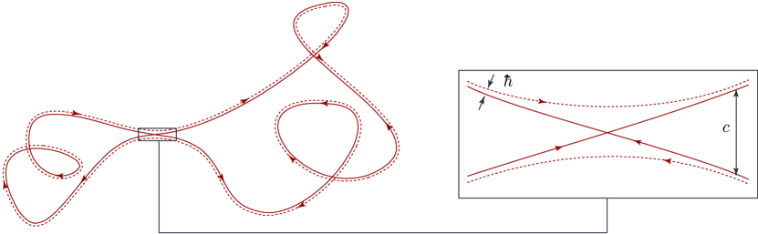
Figure 1: Cartoon of a pair of topologically distinct paths, $(\gamma,\gamma^{\prime})$ contributing to the first quantum correction to the spectral form factor. Notice that $\gamma$ and $\gamma^{\prime}$ differ in exactly one intersection point (crossing vs. avoided crossing). Inset: blow–up of the intersection region.

All corrections to the leading contribution $K^{(1)}$ hinge on the mechanism of quantum interference alluded to in the introduction. E.g., the sub–dominant contribution, $K_{\rm sc}^{(2)}$, to the form factor is provided by pairs $(\gamma,\gamma^{\prime})$ that are nearly identical except for one ‘encounter region’: In this region one of the path self–intersects while its partner just so avoids the intersection (cf. figure 1). (Alternatively, one may think of two trajectories that start out nearly identical, then split up and later recombine to form an interfering Feynman amplitude pair.) The two paths are, thus, topologically distinct yet may carry almost identical classical action [14]. Specifically, Sieber and Richter [5] have shown that for sufficiently shallow self intersections (crossing angle in configuration space of ${\cal O}(\hbar)$) the action difference $|S_{\gamma}-S_{\gamma^{\prime}}|\lesssim\hbar$. For these angles, the duration of the encounter process is of the order of the Ehrenfest time $t_{\rm E}=\lambda^{-1}\ln(c^{2}/\hbar)$, where $\lambda$ is the phase space average of the dominant Lyapunov exponent of the system and $c$ a classical reference scale (see below) whose detailed value is of secondary importance. This identifies $t_{\rm E}$ as the minimal time required to form quantum corrections to the form factor (as well as to other physical observables [14]). Throughout we shall assume $t_{\rm erg}<t_{\rm E}<t<t_{\rm H}$, where the condition $t_{\rm erg}<t_{\rm E}$ is imposed to guarantee that for time scales $t>t_{\rm E}$, the system indeed behaves universally. (For $t_{\rm erg}>t_{\rm E}$, the time window $t_{\rm E}<t<t_{\rm erg}$ is characterized by the prevalence of correlations that are non–universal yet quantum mechanical in nature.)

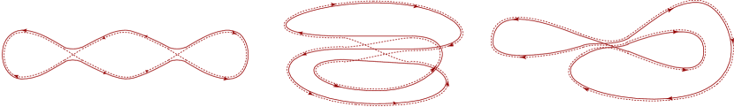
Figure 2: Cartoon of three classes of orbit pairs that contribute to the expansion of the form factor at order $\tau^{3}$. (The triple–encounter region shown in the two figures on the right is the analog of the Hikami hexagon familiar from the impurity diagram approach to disordered systems.) The existence of the middle pair does not rely on time reversal invariance.

Summation over all Sieber–Richter pairs [5] leads to the universal result $K_{\rm sc}\simeq K^{(1)}_{\rm sc}+K^{(2)}_{\rm sc}=2\tau-2\tau^{2}$, which is consistent with the short time expansion of the random matrix form factor

$$K_{\rm RM}(\tau)\stackrel{{\scriptstyle 0\leq\tau\leq 1}}{{=}}2\tau-\tau\ln(1+2\tau).$$ (2.3)

At higher orders in the $\tau$–expansion, orbit pairs of more complex topology enter the stage. (For some families of pairs contributing to the next leading correction, $K^{(3)}$, see figure 2.) The summation over all these pairs [11] — feasible under the presumed condition $t_{\rm erg}<\tau$ — obtains an infinite $\tau$–series which equals the series expansion of the RMT result (2.3). It is also noteworthy that both the topology of the contributing orbit pairs and the combinatorial aspects of the summation are in one–to–one correspondence to the impurity–diagram expansion [21] of the spectral correlation function of disordered quantum systems.

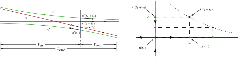
Figure 3: The structure of the encounter region. The picture on the right shows how the parallelogram spanned by the four points evolves in time $t_{1}$, while its symplectic area $us$ is conserved.

Central to our comparison of semiclassics and field theory below will be the understanding of the encounter regions where formerly pairwise aligned orbit stretches reorganize. The analysis of these objects is greatly facilitated by switching from the configuration space representation originally used in [5] to one in phase space [7, 8, 9]. In the following we briefly discuss the phase space structure of the regions where periodic orbits meet. In section 3.4 we will compare these structures to the — somewhat different — field theoretical variant of encounter processes.

Considering the correction $K_{\rm sc}^{(2)}$ as an example, we note that the encounter region contains four orbit stretches in close proximity to each other (cf. figures 1, 3): two segments ${\bf x}(t_{1})$ and ${\bf x}^{\prime}(t_{1})$ of the orbits $\gamma$ and $\gamma^{\prime}$ traversing the encounter region and the time reversed ${\bf x}(t_{1}+t_{2})$ and ${\bf x}^{\prime}(t_{1}+t_{2})$ of the trajectories reentering after one of the loops adjacent to the encounter region has been traversed ($t_{2}$ is the duration of the loop traversal and $t_{1}$ parameterizes the time during which the encounter region is passed). To describe the dynamics of these trajectory segments, it is convenient to introduce a Poincaré surface of section ${\cal S}$ transverse to the trajectory ${\bf x}(t_{1})$. For a system with two degrees of freedom (a billiard, say), ${\cal S}$ is a two–dimensional plane slicing through the three–dimensional subspace of constant energy in phase space. We chose the origin of ${\cal S}$ such that it coincides with ${\bf x}(t_{1})$. Introducing coordinate vectors ${\bf e}_{u}$ and ${\bf e}_{s}$ along the stable and unstable direction in ${\cal S}$, the three points $\bar{{\bf x}}(t_{1}+t_{2})$, ${\bf x}^{\prime}(t_{1})$ and $\bar{{\bf x}}^{\prime}(t_{1}+t_{2})$ are then represented by the coordinate pairs $(u,s),(u,0)$ and $(0,s)$, respectively. (Notice that the trajectory ${\bf x}^{\prime}$/$\bar{{\bf x}}^{\prime}$ traverses the encounter region on the unstable ($s=0$)/stable $(u=0)$ manifold thus deviating from/approaching the reference orbit ${\bf x}$.)

The above coordinate system is optimally adjusted to a description of the two main characteristics of the encounter region: its duration $t_{\rm enc}$ and the action difference $S_{\gamma}-S_{\gamma^{\prime}}$. Indeed, it is straightforward to show that the total action difference is simply given by the area of the parallelogram spanned by the four reference points in phase space, $S_{\gamma}-S_{\gamma^{\prime}}=us$ [9]. As for the encounter duration, let us assume that the distance between the orbit points may grow up to a value $c$ before they leave what we call the ‘encounter region’. (It is natural to identify $c$ with the typical phase space scale up to which the dynamics can be linearized around ${\bf x}(t_{1})$, however, any other classical scale will be just as good.) After the trajectory ${\bf x}$ has entered the encounter region, it takes a time $t_{\rm in}\sim\lambda^{-1}\ln(c/s)$ to reach the surface of section and then a time $t_{\rm out}\sim\lambda^{-1}\ln(c/u)$ to continue to the end of the encounter region. (Here, $\lambda$ is the Lyapunov exponent of the system. Thanks to the assumption $t_{\rm erg}\ll t_{\rm E}$, $\lambda$ may be assumed to be a ‘self averaging quantity’, constant in phase space.) The total duration of the passage is thus given by $t_{\rm enc}(u,s)\equiv t_{\rm out}+t_{\rm in}\sim\lambda^{-1}\ln(c^{2}/(us))$. The action difference of orbit pairs contributing significantly to the double sum must be small, $|S_{\gamma}-S_{\gamma^{\prime}}|=us\lesssim\hbar$. Consequently, $t_{\rm enc}\gtrsim t_{\rm E}\equiv\lambda^{-1}\ln(c^{2}/\hbar)$, where $t_{\rm E}$ is the Ehrenfest time introduced above. (Notice that both $S_{\gamma}-S_{\gamma^{\prime}}$ and $t_{\rm enc}$ depend only on the product $us$. While the individual coordinates $u$ and $s$ depend on the positioning of the surface of section, their product $us$ is a canonical invariant and, therefore, independent of the choice of ${\cal S}$.)

Having discussed the microscopic structure of the encounter region, we next need to ask a question of statistical nature: given a long periodic orbit $\gamma$ of total time $t$, what is the number $N(u,s,t)duds$ of encounter regions with Poincaré parameters in $[u,u+du]\times[s,s+ds]$? (To each of these encounter regions there will be exactly one topologically distinct partner orbit $\gamma^{\prime}$ that is identical to $\gamma$ in all other $(N-1)$ encounters. Thus, $N(u,s,t)duds$ is the number of Sieber–Richter pairs for a given parameter configuration and $\int\rmd u\rmd sN(u,s,t)$ is the total number of Sieber–Richter pairs.) Since the times $t_{1}$ and $t_{2}$ defining the two traversals of the encounter region are arbitrary (except for the obvious condition $|t_{1}-t_{2}|>t_{\rm enc}$), $N$ is proportional to the double integral $N(u,s,t)duds\propto{1\over 2}\int_{0,|t_{2}-t_{1}|>t_{\rm enc}}^{t}dt_{1}dt_{2}\,P_{\rm ret}(u,s,t_{2})duds$. The integrand, $P_{\rm ret}$ is the probability to propagate from the point $(0,0)$ in the Poincaré section to the time–reverse of $(u,s)$ in time $t_{2}$. Since $t_{2}>t_{\rm E}>t_{\rm erg}$, this probability is constant and equals the inverse of the volume $\Omega=2\pi\hbar t_{\rm H}$ of the energy shell, $P_{\rm ret}(u,s,t_{2})=\Omega^{-1}$. Thanks to the constancy of $P_{\rm ret}$, the temporal integrals can be performed and we obtain $N(u,s,t)\propto t(t-2t_{\rm enc})/2\Omega$. The normalization of $N$ is fixed by noting that the temporal double integral weighs each encounter event with a factor $t_{\rm enc}$. The appropriately normalized number of encounters thus reads $N(u,s)={t(t-2t_{\rm enc})\over 2t_{\rm enc}\Omega}$. Substitution of $N(u,s,t)$ into the Gutzwiller sum obtains

$$\eqalign{K^{(2)}(\tau)&=\sum_{\gamma}|A_{\gamma}|^{2}\delta\Bigl{(}\tau-{t_{\gamma}\over t_{\rm H}}\Bigr{)}\int_{-c}^{c}duds\,N(u,s,t)2\cos(us/\hbar)\\ &={\tau^{2}\over 2\pi\hbar}\int_{-c}^{c}duds\,\Bigl{(}{t\over t_{\rm enc}(u,s)}-2\Bigr{)}\cos(us/\hbar)\stackrel{{\scriptstyle\hbar\to 0}}{{=}}-2\tau^{2},}$$

where we used the sum rule $\sum_{\gamma}|A_{\gamma}|^{2}\delta(\tau-{t_{\gamma}\over t_{\rm H}})=\tau$ of Hannay and Ozorio de Almeida [22] and noted that in the semiclassical limit the first term in the integrand does not contribute (due to the singular dependence of $t_{\rm enc}$ on $\hbar$.)

Before leaving this section, let us discuss one last point related to the semiclassical approach: the analysis above hinges on the ansatz made for the classical transition probability $P_{t}({\bf x},{\bf x}^{\prime})$ between different points in phase space. Specifically, a naïve interpretation of ergodicity — $P_{t}({\bf x},{\bf x}^{\prime})=\Omega^{-1}={\rm const.}$ for times $t>t_{\rm erg}$ — is too crude to obtain a physically meaningful picture of weak localization. One rather has to take into account that the unstable coordinate, $u(t)$, separating two initially close ($u(0)\ll c$) points ${\bf x}$ and ${\bf x}^{\prime}$ grows as $u(t)\sim u(0)\exp(\lambda t)$. For sufficiently small initial separation, the time it takes before the region of local linearizability is left,

$${\textstyle\frac{1}{2}}t_{\rm E}({\bf x},{\bf x}^{\prime})\equiv\frac{1}{\lambda}\ln\frac{c}{u(0)},$$ (2.4)

may well be larger than $t_{\rm erg}$. This is important because during the process of exponential divergence, the probability to propagate from ${\bf x}$ to the time–reverse $\bar{\bf x}^{\prime}$ is identically zero. (Simply because the proximity of ${\bf x}$ and ${\bf x}^{\prime}$ implies that ${\bf x}$ and $\bar{{\bf x}}^{\prime}$ are far away from each other.) Only after the domain of linearizable dynamics has been left, this quantity becomes finite and, in fact, constant:

$$P_{t}({\bf x},{\bf x}^{\prime})={1\over\Omega}\Theta(t-t_{\rm E}({\bf x},{\bf x}^{\prime})).$$ (2.5)

This concludes our brief survey of the semiclassical approach to quantum coherence. We next turn to the discussion of the field theoretical formulation and its structural parallels to the formalism above.

3 Field Theoretical Formulation

3.1 Definition of the Model

The ballistic $\sigma$–model is defined by a functional integral ${\cal Z}(\omega)=\int{\cal D}T\rme^{-S[T]}$ extending over field configurations $T({\bf x})$ in classical phase space. Its action is given by $S[T]=S_{0}[T]+S_{\rm reg}[T]$, where

$$S_{0}[T]=\frac{\rmi}{4\hbar}\int(d{\bf x})\,\tr\Bigl{(}\frac{\omega^{+}}{2}\sigma_{3}^{\rm ar}T^{-1}\Lambda T+T^{-1}\Lambda[H,T]\Bigr{)}$$ (3.1)

is the action of the ‘native’ model [13] and $S_{\rm reg}$ a regulatory contribution to be discussed momentarily. Here, $\int(d{\bf x})\equiv(2\pi\hbar)^{-f+1}\int\rmd{\bf x}\,\delta(E_{0}-H({\bf x}))$ is the integral over the $(2f-1)$–dimensional shell $\Omega$ of constant energy $E_{0}$, $T=T({\bf x})$, $\sigma_{3}^{\rm ar}$ and $\Lambda$ are matrices whose internal structure will be discussed momentarily, $H$ the classical Hamilton function of the system, and $\omega$ the scale at which we are probing the spectrum. (Within the field theoretical approach it is preferable to work in energy rather than in time space.) Importantly, all products appearing in the action (3.1) have to be understood as Moyal products,

$$(fg)({\bf x})\equiv\rme^{\frac{\rmi\hbar}{2}\partial_{{\bf x}_{1}}I\partial_{{\bf x}_{2}}}f({\bf x}_{1})g({\bf x}_{2})\big{|}_{{\bf x}_{1}={\bf x}_{2}={\bf x}},$$

where the matrix $I$ is defined through ${\bf x}^{T}I{\bf x}^{\prime}\equiv{\bf q}\cdot{\bf p}^{\prime}-{\bf p}\cdot{\bf q}^{\prime}.$ For later reference we note that the Moyal product affords the alternative representation

$$(fg)({\bf x})=\int\frac{d{\bf x}_{1}}{(\pi\hbar)^{f}}\frac{d{\bf x}_{2}}{(\pi\hbar)^{f}}\,\rme^{\frac{2\rmi}{\hbar}{\bf x}_{1}^{T}I{\bf x}_{2}}f({\bf x}+{\bf x}_{1})g({\bf x}+{\bf x}_{2}).$$ (3.2)

Equation (3.2) makes the ‘non–locality’ inherent to the action of the ballistic $\sigma$–model manifest: all products involve a coordinate averaging over Planck cells of volume $\sim\hbar^{f}$. As we shall see below, this non–locality encapsulates essential aspects of the semiclassical dynamics discussed in the previous section.

The second contribution to the action

$$S_{\rm reg}[T]=\frac{g_{\rm reg}}{8}\int(d{\bf x})\,\tr\bigl{(}\partial_{i}T({\bf x})\partial_{i}T^{-1}({\bf x})\bigr{)}$$ (3.3)

serves to damp out singular field configurations (Unlike with most other field theories, the action of the unregularized model, governed by the generator $[H,\;]$ of unitary quantum dynamics, does not have the capacity to self–regularize.) In A we will argue that a coupling constant $g_{\rm reg}\sim\hbar^{2}$ suffices to stabilize the theory. Coupled to the theory at this strength, the action $S_{\rm reg}$ does not yet influence the dynamics on the physically relevant times $t_{\rm E}$. This stands in contrast to the theory of AL where a second order derivative term (similar in structure to (3.3) but with coupling constant $g_{\rm reg}\sim\hbar$) actively governed the dynamics at times $t\simeq t_{\rm E}$.

In the original references, the ballistic $\sigma$–model was introduced as a supersymmetric field theory. However, for the purposes of our present analysis it will be more convenient to employ the simpler formalism of the replica trick. Within this approach, the matrices $T({\bf x})\in{\rm Sp}(4R)/{\rm Sp}(2R)\times{\rm Sp}(2R)$ act in a tensor product of $R$–dimensional replica space, a two–dimensional space distinguishing between advanced and retarded propagators (ar–space) and a two–dimensional space (tr–space) whose presence is required to account for the time reversal invariance of the system [24]. Here, ${\rm Sp}(2R)$ is the $2R$–dimensional symplectic group and $\Lambda=\sigma_{3}^{\rm ar}\otimes\mathbf{1}^{\rm tr}\otimes\mathbf{1}_{R}$, where $\mathbf{1}_{R}$ is the $R$–dimensional unit matrix. While the use of replicas bars us from performing non–perturbative calculations, it significantly facilitates the comparison to the semiclassical analysis above.

3.2 Two–Level Correlation function

Our goal is to compute the two–level correlation function $R_{2}(\omega)$. Expressed in terms of single particle Green functions $G^{\pm}=(E\pm\rmi 0-H)^{-1}$,

$$R_{2}(\omega)={\Delta^{2}\over 2\pi^{2}}{\rm Re}\,\left\langle{\rm tr}(G^{+}(E+\omega/2))\,{\rm tr}(G^{-}(E-\omega/2))\right\rangle_{E,{\rm c}},$$

where $\langle\dots\rangle_{E,{\rm c}}$ denotes the (connected) average over an energy interval much larger than the inverse of the smallest time scales in the problem (the inverse of the Lyapunov time, say.) Within the replica formalism, $R_{2}$ is obtained by a two–fold differentiation of the partition function w.r.t. the energy parameter:

$$R_{2}(s)=-{\textstyle\frac{1}{2}}\lim_{R\to 0}{1\over R^{2}}{\,\rm Re}\,\partial^{2}_{s}Z(s),$$

where the dimensionless variable $s=\pi\omega/\Delta$. As long as we restrict ourselves to perturbative operations, i.e. an expansion of the two–level correlation function in a series

$$R_{2}(s)\stackrel{{\scriptstyle s>1}}{{=}}{\rm Re}\,\sum_{n=2}^{\infty}c_{n}(\rmi s^{+})^{-n},$$ (3.4)

the replica limit $R\to 0$ is well–defined. A straightforward Fourier transformation, $K(\tau)=\pi^{-1}\int\rmd s\,\rme^{-2\rmi s\tau}R_{2}(s)$, shows that the coefficients $c_{n}$ are related to the coefficients $d_{n}$ of the spectral form factor $K(\tau)\equiv\sum_{n=1}^{\infty}d_{n}\tau^{n}$ through

$$d_{n}=-\frac{(-2)^{n}}{n!}c_{n+1}.$$ (3.5)

In fact, however, there are much more far–reaching analogies between the temporal and the frequency representation of spectral correlations: at every given order $n$ various topologically distinct families of orbit/partner orbit pairs (‘diagrams’) contribute to the coefficient $d_{n}$. Likewise, the expansion coefficients $c_{n}$ obtain as sums of Wick contractions of the generating functional $Z(\omega)$. We shall see that there is an exact correspondence between field theoretical and semiclassical diagrams (both in topological structure and numerical value) which simply means that the two approaches describe spectral correlations in terms of the same semiclassical interference processes.

3.3 Quadratic Action

We next turn to the actual expansion of the field integral. For this purpose, we shall employ the so–called ‘rational parameterization’ of the coset–valued field $T$. This parameterization is defined by $T=\mathbf{1}+W$, where

$$W=\left(\matrix{&-B^{\dagger}\\ \cr B&}\right)_{\rm ar}$$ (3.6)

is a matrix that anti–commutes with the matrix $\Lambda$ introduced above. Its off–diagonal blocks take values in the Lie algebra of ${\rm Sp}(2R)$, i.e. they satisfy the constraint $B^{\dagger}=B^{\tau}\equiv(\rmi\sigma_{2}^{\rm tr}\otimes\mathbf{1}_{R})B^{T}(\rmi\sigma_{2}^{\rm tr}\otimes\mathbf{1}_{R})^{-1}$. The principal advantage of the rational parameterization is that the Jacobian associated to the transformation from the $T$–matrices to the linear space of $B$–matrices is unity: $\int{\cal D}T=\int{\cal D}B$.

Substituting this representation into the action, we obtain a series $S[B]=\sum_{n=1}^{\infty}S^{(2n)}[B]$, where $S^{(2n)}$ is of $2n$–th order in $B$. Let us begin by discussing the unregularized quadratic action

$$S_{0}^{(2)}[B]=-\frac{\rmi}{2\hbar}\int(d{\bf x})\,\tr\left[B^{\dagger}\left(\omega^{+}-[H,\;]\right)B\right],$$

where $[H,\;]$ is the generator of quantum time evolution. Very little can be said about this generator in concrete terms which means that the action $S_{0}^{(2)}$ does not qualify as a ‘reference point’ of a perturbative expansion scheme. (Indeed, notice that the projection $|\alpha\rangle\langle\alpha|$ onto an eigenstate $|\alpha\rangle$ of the Hamilton operator $H$ is annihilated by $[H,\;]$. This means that the quantum evolution operator possesses a large number of (nearly) unstable ‘zero modes’ whose action is damped only by the frequency parameter $\omega$.)

Much more is known about the generator $\{H,\,\}$ of classical dynamics, where $\{f,g\}({\bf x})\equiv\partial_{{\bf x}_{1}}^{T}I\partial_{{\bf x}_{2}}f({\bf x}_{1})g({\bf x}_{2})\big{|}_{{\bf x}_{1}={\bf x}_{2}={\bf x}}$ is the Poisson bracket. Expanding the Moyal commutator,

$$[H,B]({\bf x})=\rmi\hbar\{H,B\}({\bf x})+{\cal O}((\hbar\partial_{\bf x})^{3}B({\bf x})),$$

we notice that the quantum generator $[H,\;]$ differs from its classical counterpart $\{H,\;\}$ by the presence of higher order derivative terms. In A it is shown that the quadratic regulatory action

$$S_{\rm reg}^{(2)}[B]=g_{\rm reg}\int(d{\bf x})\,\tr\bigl{(}\partial_{i}B^{\dagger}({\bf x})\partial_{i}B({\bf x})\bigr{)}$$

suffices to damp out higher derivatives and hence effectively projects the quadratic action onto its classical limit. Assuming regularization in the above sense, our further discussion will be built on the action

$$S_{\rm cl}^{(2)}[B]={\textstyle\frac{1}{2}}\int(d{\bf x})\,\tr\left[B^{\dagger}({\bf x})({\cal L}_{\omega}B)({\bf x})\right],$$ (3.7)

where ${\cal L}_{\omega}\equiv-\rmi\omega/\hbar-\{H,\;\}$. Throughout, the operator $P_{\omega}\equiv{\cal L}_{\omega,{\rm reg}}^{-1}$ will play an important role. Here, the subscript ‘reg’ indicates that $\mathcal{L}_{\omega}$ acts in a space of functions coarse grained over cells in phase space of ‘volume’ $(\hbar^{2}/a)^{f}$, where $a$ is some classical reference scale of dimensionality ‘action’ whose detailed value will not be of much concern. Importantly, $P_{\omega}$ is not strictly inverse to the bare Liouville operator (i.e. the Liouville operator acting in the space of unregularized functions.), $\mathcal{L}_{\omega}P_{\omega}({\bf x},{\bf x}^{\prime})\not=\delta({\bf x}-{\bf x}^{\prime})$. Rather, the time Fourier transform, $P_{t}({\bf x},{\bf x}^{\prime})=\delta({\bf x}-{\bf x}(t))$ can resolve the definite dynamical evolution generated by the Liouville operator only up to time scales

$$\tilde{t}_{\rm E}\equiv\lambda^{-1}\ln\frac{c^{2}a}{\hbar^{2}}\sim 2t_{\rm E}.$$

Thereafter, the uncertainty in the resolution of the boundary conditions (the effect of smoothening) renders the dynamics unpredictable, i.e.

$$P_{t}({\bf x},{\bf x}^{\prime})=\left\{\begin{array}[]{ll}\delta({\bf x}-{\bf x}^{\prime}(t))&,\ t<\tilde{t}_{\rm E},\cr\Omega^{-1}&,\ t>\tilde{t}_{\rm E}.\end{array}\right.$$ (3.8)

the crossover between the two regimes takes place over time scales $\sim\max\{\Delta\tilde{t}_{\rm E},t_{\rm erg}\}$, where $\Delta\tilde{t}_{\rm E}\ll t_{\rm E}$ is the uncertainty in $\tilde{t}_{\rm E}$ caused by an eventual non–uniformity of the Lyapunov expansion. (Notice that in previous discussions of the ballistic $\sigma$–model, the propagator $P$ was mostly identified with the Perron–Frobenius operator, i.e. an object that describes relaxation into a uniform configuration, $P_{t}({\bf x},{\bf x}^{\prime})\stackrel{{\scriptstyle t>t_{\rm erg}}}{{=}}{\rm const.}$ over classically short times. However, it is not at all clear how this behaviour may be reconciled with the indispensable condition that $P_{t}({\bf x},\bar{\bf x}^{\prime})\stackrel{{\scriptstyle t<t_{\rm E}({\bf x},{\bf x}^{\prime})}}{{=}}0$: for $|{\bf x}-{\bf x}^{\prime}|={\cal O}(\hbar)$, the propagator must be able to resolve fine structures in phase space over times $\sim t_{\rm E}$ parametrically larger than the relaxation time of the Perron–Frobenius operator. In contrast, equation (3.8) is motivated by the structure of the action, and does resolve the classical phase space dynamics up to the Ehrenfest time. In fact, we will see that the scale $\tilde{t}_{\rm E}>t_{\rm E}$ does not explicitly enter the results of the theory. The reason is that, due to a conspiracy of quantum non–locality and chaotic instability, the dynamics becomes effectively irreversible instantly after the Ehrenfest time (on time scales of the order of the inverse Lyapunov exponent). Thus, at a time where the artificially introduced smearing would become virulent, the theory has long become quantum–unpredictable.)

3.4 Perturbative Expansion

We now have everything in store to proceed to the perturbative expansion of the functional integral. The dominant contribution to the series (3.4) obtains by integration over the quadratic action:

$$\eqalign{R_{2}^{(2)}(s)&=-{\textstyle\frac{1}{2}}\lim_{R\to 0}{1\over R^{2}}{\rm Re}\,\partial_{s}^{2}\int{\cal D}B\exp(-S_{\rm cl}[B])\\ &=-{\textstyle\frac{1}{2}}\,{\rm Re}\lim_{R\to 0}{1\over R^{2}}\partial_{s}^{2}(\det P_{\omega})^{2R^{2}}={\rm Re}\,\partial_{s}^{2}\ln\det(P^{-1}_{\omega})\stackrel{{\scriptstyle\omega\ll\hbar/t_{\rm erg}}}{{\simeq}}{\rm Re}\,(\rmi s^{+})^{-2}.}$$ (3.9)

This result implies (cf. equations (3.4, 3.5)) $d_{1}=2$ in accord with the semiclassical analysis.

To compute higher order terms in the expansion we need to consider the non–linear contributions $S^{(2n>2)}$ to the action. Substituting the representation (3.6) into the action (3.1) we obtain

$$S^{(2n)}[B]={\textstyle\frac{1}{2}}\int(d{\bf x})\tr\left[(-B^{\dagger}B)^{n-1}B^{\dagger}\mathcal{L}_{\omega}B\right].$$ (3.10)

By elementary power counting, each matrix $B$ scales as (symbolic notation) $\sim(\mathcal{L}_{\omega})^{-\frac{1}{2}}\sim\omega^{-\frac{1}{2}}\sim s^{-\frac{1}{2}}$. This implies that each vertex $S^{(2n)}$ contributes a factor $\sim(B^{\dagger}B)^{n-1}B^{\dagger}\mathcal{L}_{\omega}B\sim s^{-n+1}$ to the functional integral. Specifically, the dominant correction ($\sim s^{-3}$) to the leading contribution (3.9) obtains by first order expansion in the vertex $S^{(4)}$:

$$R_{2}^{(3)}(s)=-{\,\rm Re}\lim_{R\to 0}\frac{1}{(2R)^{2}}\partial^{2}_{s}\int(d{\bf x})\langle{\,\rm tr}(B^{\dagger}BB^{\dagger}\mathcal{L}_{\omega}B)\rangle_{B}.$$ (3.11)

We emphasize again that all products of $B$–matrices have to be understood as Moyal products. To obtain a convenient representation of the product of more than two of these matrices, we iteratively apply the prototype formula equation (3.2). A straightforward calculation then yields the general product formula

$$(A_{1}\dots A_{2n})({\bf x})=\int\prod_{i=1}^{2n}\frac{d{\bf x}_{i}}{(\pi\hbar)^{f}}\,\rme^{\frac{\rmi}{\hbar}S({\bf x}_{1},\cdots{\bf x}_{2n})}A_{1}({\bf x}+{\bf x}_{1})\dots A_{2n}({\bf x}+{\bf x}_{2n}),$$

where the bilinear form $S({\bf x}_{1},\cdots{\bf x}_{2n})\equiv 2\sum_{i<j}(-)^{i+j}{\bf x}_{i}^{T}I{\bf x}_{j}$. Below, we will apply this formula to the fields $B$ of the theory. In A we show that in this case, all energy coordinates $E_{i}$ get locked. Here, we assume a coordinate choice ${\bf x}=(E,t,{\bf y})$ where $E$ is an energy variable, $\tau$ its canonically conjugate time–like variable (a coordinate parameterizing the Hamiltonian flow through ${\bf x}$) and ${\bf y}$ a $(2f-2)$–dimensional vector of coordinates transverse to the flow. Further, fluctuations in the time–like variables $\tau_{i}$ are negligible. Introducing the shorthand notation $\int_{{\bf x}_{i}}\equiv(\pi\hbar)^{-f+1}\int\rmd{\bf x}_{i}\,\delta(E_{i}-E_{0})\delta(\tau_{i})$, we thus have

$$(B^{\dagger}B)^{2n}({\bf x})=\int_{{\bf x}_{1},\dots,{\bf x}_{2n}}\rme^{\frac{\rmi}{\hbar}S({\bf x}_{1},\cdots{\bf x}_{2n})}B^{\dagger}({\bf x}+{\bf x}_{1})\dots B({\bf x}+{\bf x}_{2n}).$$ (3.12)

Using this representation in (3.11), applying the contraction rules (2.1) discussed in B, and taking the replica limit we obtain

$$R_{2}^{(3)}(s)={\rm Re}\Bigl{(}\frac{\Omega}{t_{\rm H}}\Bigr{)}^{2}\partial_{s}^{2}\int(d{\bf x})\int_{{\bf x}_{1},\dots,{\bf x}_{4}}\rme^{\frac{\rmi}{\hbar}S({\bf x}_{1},\dots,{\bf x}_{4})}P_{\omega}(\overline{{\bf x}+{\bf x}_{1}},{\bf x}+{\bf x}_{3}){\cal L}_{\omega,{\bf x}_{4}}P_{\omega}({\bf x}+{\bf x}_{4},\overline{{\bf x}+{\bf x}_{2}}),$$

where the coordinate subscript in ${\cal L}_{\omega,{\bf x}}$ indicates the argument on which the Liouvillian acts. The physical meaning of this expression is best revealed by switching to the Fourier conjugate picture. Inserting the definition (2.2) of the form factor, we obtain

$$\eqalign{K^{(2)}(\tau)=-2\tau^{2}&\frac{\Omega^{2}}{t_{\rm H}}\int(d{\bf x})\int_{{\bf x}_{1},\dots,{\bf x}_{4}}\rme^{\frac{\rmi}{\hbar}S({\bf x}_{1},\dots,{\bf x}_{4})}\times\\ &\times\int_{0}^{t}dt^{\prime}P_{t-t^{\prime}}(\overline{{\bf x}+{\bf x}_{1}},{\bf x}+{\bf x}_{3}){\cal L}_{t^{\prime},{\bf x}_{4}}P_{t^{\prime}}({\bf x}+{\bf x}_{4},\overline{{\bf x}+{\bf x}_{2}}),}$$ (3.13)

where $\mathcal{L}_{t}\equiv\partial_{t}-\{H,\;\}$. equation (3.13) makes the analogies (as well as a number of differences) between the semiclassical and the field theoretical description of quantum corrections explicit: central to both approaches are two semi–loops shown schematically in figure 1. In either case, the proximity of these loops is controlled by phase factors which contain the coordinates of the end points (in a canonically invariant manner) as their arguments. However, unlike with semiclassics, equation (3.13) does not relate the unification of the two semi–loops to specific periodic orbits. Rather, the two halves are treated as independent entities, each described in terms of its own probability factor $P$. Relatedly, the phase factor controlling the proximity of the terminal points does not correspond to the action difference between two orbits.

The result obtained for $K^{(2)}(\tau)$ in equation (3.13) critically depends on the behaviour of the propagator $P_{t}$ at times $t\sim t_{\rm E}({\bf x},{\bf x}^{\prime})\sim t_{\rm E}$, cf. equations (2.4, 2.5). Specifically, we shall use that $\partial_{t}P_{t}(\bar{{\bf x}},{\bf x}^{\prime})=\Omega^{-1}\delta(t-t_{\rm E}({\bf x},{\bf x}^{\prime}))$, where $\delta(t)$ is some smeared $\delta$–function whose detailed functional structure is not of much importance. (All we shall rely upon is $\int\rmd t\delta(t)f(t)\simeq f(t)$ for functions that vary slowly on the scales where $\delta(t)$ varies.) We also note that the Poisson bracket $\{H,f\}({\bf x})\sim\partial_{t}f({\bf x})$ effectively differentiates along the trajectory through ${\bf x}$. However, the time $t_{\rm E}({\bf x},{\bf x}^{\prime})=t_{\rm E}({\bf y},{\bf y}^{\prime})$ defined in equation (2.4) depends only on the coordinates transverse to the trajectory. This implies $\{H,P_{t}(\bar{{\bf x}},{\bf x}^{\prime})\}=\{H,P_{t}(t_{\rm E}({\bf x},{\bf x}^{\prime}))\}=0$. We thus conclude that the action of ${\cal L}_{t}$ on the function $P$ is given by ${\cal L}_{{\bf x},t}P_{t}(\bar{{\bf x}},{\bf x}^{\prime})\simeq\Omega^{-1}\delta(t-t_{\rm E}({\bf x},{\bf x}^{\prime}))\simeq\Omega^{-1}\delta(t-t_{E})$. To understand the meaning of the second approximation, notice that it takes a time $t_{E}$ before the bulk of the Planck cell to which the points ${\bf x}$ and ${\bf x}^{\prime}$ belong has grown to classical scales $c$. For times $t>t_{E}$, the fraction of the Planck cell which has not yet acquired macroscopic dimensions shrinks exponentially on the classical Lyapunov scale $\lambda^{-1}\ll t_{E}$. This means that $t_{E}({\bf x},{\bf x}^{\prime})\simeq t_{E}$ up to an insignificant uncertainty of ${\cal O}(\lambda^{-1})$. Using these results, as well as the normalization relations $\int(d{\bf x})=t_{\rm H}$ and $\int_{{\bf x}_{1},\dots,{\bf x}_{2n}}\rme^{\frac{\rmi}{\hbar}S({\bf x}_{1},\dots,{\bf x}_{2n})}=1$, we obtain

$$\eqalign{K^{(2)}(\tau)&\simeq-2\tau^{2}\frac{1}{t_{\rm H}}\int(d{\bf x})\int_{{\bf x}_{1},\dots,{\bf x}_{4}}\rme^{\frac{\rmi}{\hbar}S({\bf x}_{1},\dots,{\bf x}_{4})}\int_{0}^{t}dt^{\prime}\Theta(t-t^{\prime}-t_{\rm E})\delta(t^{\prime}-t_{\rm E})\\ &=-2\tau^{2}\Theta(t-2t_{\rm E})}$$

in agreement with the result of the semiclassical analysis.

3.5 Higher Orders of Perturbation Theory

What happens at higher orders in perturbation theory in the parameter $s^{-1}$? Before turning to the problem in full, it is instructive to have a look at the zero mode approximation to the model. The action of the zero mode configuration — formally obtained by setting $T({\bf x})\equiv T={\,\rm const.}$ — is given by $S_{0}[Q]=\rmi s^{+}{\rm tr}(\sigma_{3}^{\rm ar}Q)/4$, where we have used the standard [27] notation $Q\equiv T^{-1}\Lambda T$. Parameterizing the matrix $T=1+W$ as in (3.6), an expansion in the generators $B$ obtains the expression

$$S_{0}[B]=\sum_{n=1}^{\infty}S_{0}^{(2n)}[B],\qquad S_{0}^{(2n)}[B]=-\rmi s^{+}{\rm tr}(-B^{\dagger}B)^{n}.$$ (3.15)

It is known [27] that, term by term in an expansion in $s^{-1}$, the zero mode functional reproduces the RMT approximation to the correlation function $R_{2}(s)$. Second, there exists a far–reaching structural connection between the perturbative expansion of the zero mode theory on the one hand and the Gutzwiller double sum on the other. (In fact, the correspondence Gutzwiller sum $\leftrightarrow$ zero dimensional $\sigma$–model $\leftrightarrow$ RMT played a pivotal role in the proof that the semiclassical expansion coincides with the RMT result. [11])

More specifically, to each term contributing to the Wick contraction of

$$\langle(S_{0}^{(4)}[B])^{m_{2}}\,(S_{0}^{(6)}[B])^{m_{3}}\dots\rangle_{0}$$ (3.16)

there corresponds precisely one semiclassical orbit/partner orbit pair (or ‘diagram’). By power counting, this diagram contributes to the correlation function at order $s^{-2-\sum_{n}m_{n}(n-1)}$. For every value of $n=2,3,\dots$, it contains $m_{n}$ encounter regions where $n$ orbit segments meet and $\sum_{n}nm_{n}$ inter-encounter orbit stretches. The topology of the diagram is fixed by the way in which the $B$ matrices are contracted. (For example, the first of the diagrams shown in figure 2 corresponds to the contraction $(1-3,2-6,4-8,5-7)$ of ${\rm tr}(B^{\dagger}BB^{\dagger}B)\,{\rm tr}(B^{\dagger}BB^{\dagger}B)$, the second diagram to the contraction $(1-4,2-5,3-6)$ of ${\rm tr}(B^{\dagger}BB^{\dagger}BB^{\dagger}B)$, etc.) Importantly, the minimum time required for the buildup of a diagram (i.e., the time required to traverse the $\sum_{n}m_{n}$ encounter regions) is given by $t_{\rm E}\times\sum_{n}nm_{n}$.

Turning back to the full problem, let us consider the analog of the zero dimensional expression (3.16),

$$\langle(S^{(4)}[B])^{m_{2}}\,(S^{(6)}[B])^{m_{3}}\dots\rangle,$$ (3.17)

where $S^{(2n)}$ is given by (3.10) and the average is over the full quadratic action (3.7). It is natural to expect that the unique correspondence between Wick contractions and semiclassical diagrams carries over to the full model. If so, individual contractions should vanish/reduce to the universal RMT result for times shorter/much larger than $t<t_{\rm E}\times\sum_{n}nm_{n}$. In section 3.4 this correspondence was exemplified for the simplest non–trivial example, the Sieber–Richter diagram $\langle S^{(4)}[B]\rangle$.

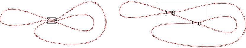
Figure 4: Two representatives of the ‘clover leaf’ diagram class contributing to the form factor at ${\cal O}(\tau^{3})$. Discussion, see text.

Perhaps unexpectedly, the straightforward one–to–one correspondence outlined above does not pertain to higher orders in perturbation theory. To anticipate our main findings, it turns out that at order $(s^{-4}\leftrightarrow\tau^{3})$ in the series expansion, propagators of short duration $P_{t<t_{\rm E}}$ — absent in the $(\tau^{2}\leftrightarrow s^{-3})$ term considered above — begin to play a role. This implies that individual contractions may relate to more than one semiclassical diagram class. Nonetheless, integration over all time parameters obtains a universal result.

By way of example, let us consider the $(1-3,2-6,4-8,5-7)$ contraction of $\langle{\rm tr}(B^{\dagger}BB^{\dagger}B){\rm tr}(B^{\dagger}BB^{\dagger}B)\rangle$. For generic values ($t_{i}\sim t_{\rm H}\gg t_{\rm E}$) of the time arguments carried by the four resulting propagators the contraction corresponds to the orbit pair shown in figure 2 left. However, the integration over times $t_{i}$ also extends over exceptional values where one of the two propagators connecting the two encounter regions ($(2-6)$ or $(4-8)$) is of short duration $<t_{\rm E}$. Such a short time propagator connects two distinct vertices. This results in a structure as shown in figure 4 right, where the two clusters of dots indicate the eight phase space arguments of the $B$–fields, the straight line–pair represents the short propagator, and the box indicates that all phase space points lie in a single encounter region. Evidently, this structure corresponds to a pair of orbits visiting a single encounter region twice. Diagrams of this structure are canonically obtained by contraction of a ‘Hikami hexagon’ ${\rm tr}(B^{\dagger}BB^{\dagger}BB^{\dagger}B)$, as indicated in figure 4 left. Fortunately, the absence of a unique assignment to semiclassical orbit families, does not significantly complicate the actual computation of the diagrams: closer inspection shows that taking the Liouville operators involved in the definition of the Hikami boxes into account and integrating by parts, we again obtain the universal zero–mode result.

Summarizing, we have seen that at next to leading order in perturbation theory short time propagators begin to play a role. While this complication prevents the assignment of Wick contractions to orbit pairs of definite topology, the results obtained after integration over all temporal configurations remain universal (agree with the RMT prediction). We trust that the structures discussed above are exemplary for the behaviour of the ballistic $\sigma$–model at arbitrary orders of perturbation theory, i.e. that after integration over all intermediate times, each contraction contributing to (3.17) produces the universal result otherwise obtained by its zero dimensional analog equation (3.16).

4 Conclusions and Outlook

In this paper, we have applied field theoretical methods to explore quantum interference corrections to the spectral form factor of individual chaotic systems. We have seen that the formation of the latter essentially relies on the fact that the ballistic $\sigma$–model — a field theory defined in classical phase space — is not capable of resolving structures on scales smaller than the Planck cell. This quantum uncertainty is an intrinsic feature of the model (viz. through the fact that the field degrees of freedom are multiplied by Moyal rather than by conventional products) and need not be added by hand as was done in previous approaches. In a manner that largely parallels the results of recent semiclassical analyses, the interplay of this uncertainty with the instabilities of the underlying classical chaotic dynamics leads to the formation of universal quantum interference corrections to the spectral form factor.

The analysis above is perturbative in nature and, thus, limited to energy scales larger than the single particle level spacing. To advance into the perturbatively inaccessible regime $\omega<\Delta$ (i.e. to prove the universality hypothesis in full) one would need to understand how the conspiracy of quantum uncertainty and classical instabilities damps out fluctuations inhomogeneous in phase space at time scales larger than the Ehrenfest time. The identification of a concrete mechanism effecting this reduction remains an open issue.

Appendix A Regularization

Throughout this appendix we use phase space coordinates ${\bf x}=(E,t,{\bf y})$, where $E$ is the energy, $t$ a time–like coordinate conjugate to energy and parameterizing the Hamiltonian flow through ${\bf x}$, and ${\bf y}$ a $(2f-2)$–component vector of energy shell coordinates transverse to $t$.

A.1 In–Shell Regularization

As discussed in the text, the quadratic action of the model is controlled by the commutator $[H,\;]$ or, upon Wigner transformation, the series of operators $[H,\;]\mapsto\rmi\hbar\{H,\;\}+\sum_{n=1}^{\infty}\hbar^{2n+1}D^{(2n+1)}(\partial_{\bf x})$, where $D^{(2n+1)}(\partial_{\bf x})$ is an operator of $(2n+1)$–th order in the phase space derivatives $\{\partial_{x_{i}}\}$. When acting in a space of functions smooth on scales $\hbar$, terms beyond the leading term (the Poisson bracket) are inessential and the quantum dynamics collapses to its semiclassical limit. Naïvely, one might hope that to achieve this reduction it suffices to choose the initial distributions in phase space sufficiently smooth. However, what complicates the problem is that the generator of classical evolution $\{H,\;\}$ by itself leads to the dynamical buildup of singularities, no matter how smooth the initial distribution was. The point is that, due to the global hyperbolicity of the dynamics, we may locally identify truly expanding and contracting coordinate directions. Focusing attention on the latter, and linearizing the flow around a given reference trajectory, the equations of motion controlling the evolution of a phase space distribution $\rho$ assume the form $\dot{\rho}=\{H,\rho\}=\lambda s\partial_{s}\rho+\dots$, where $s$ is the coordinate that contracts strongest, $\lambda$ the corresponding Lyapunov exponent, and the ellipses indicate derivatives in other coordinate directions. After a time $t\sim\lambda^{-1}\ln(\delta x_{0}/\hbar)$, where $\delta x_{0}$ denotes the characteristic initial extension of the distribution, structures in the $s$–direction fluctuating on scales $\lesssim\hbar$ will have formed implying that derivatives $D^{(2n+1)}$ acting in $s$–direction can no longer be neglected. One way to remove this complication [28] is to add to the generator of classical time evolution an elliptic operator $\sim D\partial_{s}^{2}$, where $D$ is constant. Indeed, it is straightforward to show (by dimensional analysis or by explicit calculation) that for the regularized operator $\lambda s\partial_{s}+D\partial^{2}_{s}$ the initial contraction halts at a characteristic scale $s\sim(D/\lambda)^{\frac{1}{2}}$. Choosing $D\sim\hbar^{2}$, it is guaranteed that the distribution will not build up structure on scales $<\hbar$, i.e. that the quantum corrections to classical dynamics are negligible. This motivates the addition of the regulatory contribution (3.3) to the action.

A.2 Off–Shell Regularization

In the main text (cf., e.g., equation (3.12)), we have assumed that (a) all fields are defined on a shell of constant energy $E_{0}$ and (b) the theory is local in the conjugate ‘time’ coordinate $t$. To understand the meaning of this reduction, we need to recall the original definition of the field degrees of freedoms, $Q({\bf x})$, of the ballistic $\sigma$–model. According to Ref. [13], $Q=T^{-1}\tilde{\Lambda}T$, where $\tilde{\Lambda}\equiv\delta_{E_{\rm av}}(E_{0}-H)\otimes\Lambda$ and the ‘delta function’

$$\delta_{E_{\rm av}}(E_{0}-H)\equiv\frac{1}{\pi E_{\rm av}}\sqrt{1-\Bigl{(}\frac{E_{0}-H}{2E_{\rm av}}\Bigr{)}^{2}}$$

projects on an energy window of width $E_{\rm av}$. (In the original reference, $E_{\rm av}$ was identified with the energy window over which the two–point correlation function (2.1) is averaged, hence the subscript ‘av’.) Integrating an action functional of these field degrees of freedom over all of phase space and absorbing $\delta_{E_{\rm av}}$ into the integration measure, $d{\bf x}\mapsto d{\bf x}\times\delta_{E_{\rm av}}(E_{0}-H)\propto(d{\bf x})$, we obtain the ‘energy shell’ measure used in the text. To understand the energy dependence of the fields themselves, we write $T({\bf x})=1+W({\bf x})$, where $W({\bf x})$ anti–commutes with $\Lambda$ and, therefore, commutes with the function $\delta_{\rm E_{\rm av}}(E_{0}-H)$. (Recall that all products are Moyal products, i.e. functions in phase space do not necessarily commute with each other.) Evaluating the latter condition, we obtain $[W,\delta_{E_{\rm av}}(E_{0}-H)]({\bf x})=\rmi\hbar\delta^{\prime}_{E_{\rm av}}(E_{0}-E)\partial_{t}W+{\cal O}(\hbar^{3})$. To rigorously fulfill this condition, we would need to require independence of $W$ of the coordinate $t$ along the flow through the phase space point ${\bf x}$ — obviously too strong a restriction. Instead, we will impose the weaker condition of approximate commutativity, $||[W,\delta_{E_{\rm av}}(E_{0}-H)]||^{2}\ll||W\delta_{E_{\rm av}}(E_{0}-H)||^{2}$, where the operator norm is defined as $||A||^{2}\equiv{\rm tr}(A^{\dagger}A)=\int\rmd{\bf x}|A({\bf x})|^{2}$. It is straightforward to check — by explicit calculation or by dimensional reasoning — that the commutator is small in the above sense provided that $\partial_{t}W<(E_{\rm av}/\hbar)W$, i.e. the fields $W$ have to be smooth in ‘time direction’ on scales $\sim\hbar/E_{\rm av}$.

The above energy–time duality suggests the following interpretation of the theory: let us introduce a ‘stroboscopic’ picture of the particle dynamics wherein time scales smaller than a certain classical $t_{0}$ need not be resolved. (E.g., in a billiard, $t_{0}\ll t_{\rm f}$ where $t_{\rm f}$ is the time of flight through the system, etc.) All fields are smooth on scales $t_{0}$. This means that the width of the averaging window must be (at least) of order $E_{\rm av}\lesssim\hbar/t_{0}$. In the classical limit, we indeed project onto a sharp ‘energy shell’. (However, we do not know how to reconcile the condition of anti–commutativity with $\Lambda$ with the condition of a mathematically sharp energy shell proposed in [17].) Second, we require that the fields $W(E)$ do not vary significantly over their narrow range $[E_{0}-E_{\rm av},E_{0}+E_{\rm av}]$ of definition (the so–called ‘mode locking assumption’ [13]). This can be achieved by choosing the second order regulator derivative in $E$ direction as $\sim(\hbar/t_{0})^{2}\partial^{2}_{E}$. We thus integrate over field configurations that are coarse grained over Planck cells of extension $(t_{0},E_{\rm av}=\hbar/t_{0})$. As a result, the integral over the $(E,t)$–sector of the Moyal products can be carried out and we arrive at the theory independent of energies and local in time direction considered in the text.

Appendix B Perturbation Theory

For completeness, we briefly summarize the contraction rules [13] employed in calculating integrals over products of $B$ matrices:

$$\eqalign{\langle\tr(B({\bf x})A)\;\tr(B^{\dagger}({\bf x}^{\prime})A^{\prime})\rangle_{B}&=\frac{\Omega}{t_{\rm H}}P_{\omega}({\bf x},{\bf x}^{\prime})\,\tr(AA^{\prime}),\\ \langle\tr(B({\bf x})AB^{\dagger}({\bf x}^{\prime})A^{\prime})\rangle_{B}&=\frac{\Omega}{t_{\rm H}}P_{\omega}({\bf x},{\bf x}^{\prime})\,\tr(A)\,\tr(A^{\prime}),\\ \langle\tr(B({\bf x})A)\;\tr(B({\bf x}^{\prime})A^{\prime})\rangle_{B}&=\frac{\Omega}{t_{\rm H}}P_{\omega}({\bf x},\bar{{\bf x}}^{\prime})\,\tr(AA^{\prime\tau}),\\ -\langle\tr(B({\bf x})AB({\bf x}^{\prime})A^{\prime})\rangle_{B}&=\frac{\Omega}{t_{\rm H}}P_{\omega}({\bf x},\bar{{\bf x}}^{\prime})\,\tr(AA^{\prime\tau}).}$$ (2.1)

where $A$ and $A^{\prime}$ are arbitrary fixed matrices. To compute the integral over an arbitrary product of traces of $B$–matrices, one first forms all possible total pairings $B$—$B^{\dagger}$, $B$—$B$, and $B^{\dagger}$—$B^{\dagger}$, and then computes individual pairings by means of (2.1). Each contraction reduces the number of matrices by two. Eventually, one obtains an expression $\sim(\tr\,\mathbf{1})^{n}=(2R)^{n\geq 2}$ (where all contributions with $n>2$ vanish in the replica limit).

References

References

- [1] J. P. Keating, Nonlinearity 4, 309 (1991).
- [2] E. Bogomolny, B. Georgeot, M. J. Giannoni, and C. Schmit, Phys. Rep. 291, 219 (1997).
- [3] J. Zakrzewski, K. Dupret, and D. Delande, Phys. Rev. Lett. 74, 522 (1995).
- [4] O. Bohigas, M. J. Giannoni, and C. Schmit, Phys. Rev. Lett. 52, 1 (1984).
- [5] M. Sieber and K. Richter, Physica Scripta T90, 128 (2001).
- [6] M. Sieber, J. Phys. A 356, L613 (2002).
- [7] S. Müller, Eur. Phys. J. B 34, 305 (2003).
- [8] M. Turek and K. Richter, J. Phys. A: Math. Gen. 36, L455 (2003).
- [9] D. Spehner, J. Phys. A: Math. Gen. 36, 7269 (2003).
- [10] S. Heusler, S. Müller, P. Braun, and F. Haake, J. Phys. A: Math. Gen. 37, L31 (2004).
- [11] S. Müller, S. Heusler, P. Braun, F. Haake, and A. Altland, Phys. Rev. Lett. 93, 14103 (2004).
- [12] B. A. Muzykantskii and D. E. Khmel’nitskii, JETP Lett. 62, 76 (1995).
- [13] A. V. Andreev, B. D. Simons, O. Agam, and B. L. Altshuler, Phys. Rev. Lett. 76, 3947 (1996).
- [14] I. L. Aleiner and A. I. Larkin, Phys. Rev. B 54, 14423 (1996).
- [15] I. L. Aleiner and A. I. Larkin, Chaos, Solitons & Fractals 8, 1179 (1997).
- [16] C. Tian and A. I. Larkin, Phys. Rev. B 70, 1 (2004).
- [17] K. B. Efetov, G. Schwiete, and K. Takahashi, Phys. Rev. Lett. 92, 26807 (2004).
- [18] C. Tian, A. Kamenev, and A. Larkin, Phys. Rev. Lett. 92, 124101 (2004); C. Tian, A. Kamenev and A. Larkin, cond-mat/0412259.
- [19] M. V. Berry, Proc. R. Soc. London A 400, 229 (1985).
- [20] M. L. Mehta, Random Matrices (Academic Press, New York, 1991).
- [21] R. A. Smith, I. V. Lerner, and B. L. Altshuler, Phys. Rev. B 58, 10343 (1998).
- [22] J. H. Hannay and A. M. O. de Almeida, J. Phys. A: Math. Gen. 177, 3429 (1984).
- [23] F. Haake, Quantum Signatures of Chaos (Springer, Berlin, 2001).
- [24] F. J. Wegner, Z. Phys. B 35, 207 (1979).
- [25] V. I. Oseledec, Trans. Moscow Math. Soc. 19, 197 (1968).
- [26] A. D. Mirlin, in Proceedings of the International School of Physics “Enrico Fermi”, Course CXLII, “New Directions in Quantum Chaos”, Società Italiana di Fisica, edited by G. Casati, J. Guarneri, and U. Smilansky (IOS Press, Amsterdam, 1999), p. 224.
- [27] K. B. Efetov, Adv. Phys. 32, 53 (1983).
- [28] W. H. Zurek and J. P. Paz, Phys. Rev. Lett. 75, 2508 (1994).