Anomalous transport in Charney-Hasegawa-Mima flows

Abstract

Transport properties of particles evolving in a system governed by the Charney-Hasegawa-Mima equation are investigated. Transport is found to be anomalous with a non linear evolution of the second moments with time. The origin of this anomaly is traced back to the presence of chaotic jets within the flow. All characteristic transport exponents have a similar value around $\mu=1.75$, which is also the one found for simple point vortex flows in the literature, indicating some kind of universality. Moreover the law $\gamma=\mu+1$ linking the trapping time exponent within jets to the transport exponent is confirmed and an accumulation towards zero of the spectrum of finite time Lyapunov exponent is observed. The localization of a jet is performed, and its structure is analyzed. It is clearly shown that despite a regular coarse grained picture of the jet, motion within the jet appears as chaotic but chaos is bounded on successive small scales.

I Introduction

Understanding transport in turbulent magnetized plasma is a task of fundamental importance. In these plasma, transport problems are often related to confinement, which is one of the last standing issues confronting the realization of magnetically confined controlled fusion devices. As the literature evolves, there has been more and more evidence showing that the transport properties can be anomalous, in the sense that transport may not be correctly described by Gaussian kinetics, but by what one now calls “strange kinetics” Schlesinger93 . In these regards, transport phenomena in turbulent magnetized plasma is part of the ever growing number of physical systems displaying anomalous propertiesCarreras03 ; Annibaldi00 ; Castillo2004 ; Grandgirard2000 . As of today the full understanding of these phenomena are far from being complete and in many regards a full blown theory able to capture and describe correctly these “strange kinetics” has not yet surfaced. There seems nevertheless to be a common agreement to link these phenomena to Levy-type processes and their generalizations. Moreover the use of fractional derivatives in Fokker-Plank-Kolmogorov type equations captures qualitatively some of the transport properties and is thus a good step towards a proper description of anomalous transport Zaslavsky2002 .

The link between the Hamiltonian dynamics and the kinetics at origin of anomalous transport properties are relatively well understood when dealing with low dimensional systems such as a time periodic flow which belong to the class of $1-1/2$ degree of freedom Hamiltonians. The dynamics in these systems is not ergodic: a well-defined stochastic sea, with chaotic dynamics, filled with various islands of quasi-periodic dynamics compose the phase space. The anomalous properties and their multi-fractal nature are then linked to the existence of islands within the stochastic sea and the phenomenon of stickiness observed around them Kuznetsov2000 ; LKZ01 . However when dealing with more complex systems the loss of time-periodicity complicates the picture. For instance in geophysical flows or two-dimensional plasma turbulence, the islands which were static and well localized in phase space, are replaced by “coherent structures”, which have a life of their own. Hence, tackling the origin of anomalous transports from the chaotic dynamics of individual tracers becomes more subtle. Recently, the existence of a hidden order for the tracers which exhibits their possibility to travel in each other’s vicinity for relatively large times was exhibited LZ02 . This order is related to the presence within the system of chaotic jets Afanasiev91 ; LZ03 . These chaotic jets can be understood as moving clusters of particles within a specific domain for which the motion appears as almost regular from a coarse grained perspective. Typically, the chaotic motion of the tracers is confined within the characteristic scale of a given jet, within which nearby tracers are trapped. From another point of view, looking for chaotic jets can be understood as a particular case of measurements of space-time complexityAfraimovich03 .

The purpose of this paper is to study transport properties and to look for chaotic jets in a model of two-dimensional turbulence which applies either in the plasma context where it is known as the Hasegawa-Mima equation Hasegawa1981 or in the geophysical one where one speaks about the Charney equation (see for instance Pedlosky_book ). In this setting Annibaldi et al have already shown strong evidence of anomalous transport of passive particles Annibaldi00 ; Annibaldi02 , hence the search for chaotic jet is expected to give some clues on the origin of anomalous transport in these systems, and for instance to identify the structures responsible for such transport. Indeed in LZ02 , it was clearly shown that trapping within chaotic jets resulted in anomalous transport. Moreover it appeared that jets were localized around the coherent structures of systems, namely the vortex cores and that the structure of the jets itself was a hierarchy of jets within jets, reminiscent of the multi-fractal nature of transport observed in $1-1/2$ degree of freedom Hamiltonians systems LKZ01 . Hence, the goal of this paper may be seen as two-fold. First we want to understand the origin of anomalous transport in a model of two-dimensional plasma turbulence. And second, since we are using chaotic jets to track this origin, we are at the same time testing the existence of these jets in a more complex setting than the system of point vortices used in LZ02 . Once the presence of jets is confirmed we may be able to speculate that the different anomalous transport behavior portrayed in the nonexhaustive following references Nau99 ; Carreras03 ; Dickman04 ; Dupont98 ; Sukhatme04 ; Beyer2001 may all find their origin in the presence of long lived chaotic jets in the considered systems.

The paper is organized as follows. In Sec. II the basic definitions are introduced. A brief introduction of the Charney-Hasegawa-Mima equation is given. Then the dynamics of test particles is given and the Lagrangian approach of transport in this setting is discussed. In Sec. III the dynamical evolution of the field and of passive test particles, as well as transport properties are computed numerically. First the numerical setting is discussed. Then three different regimes corresponding to different choices of the parameters for the field evolution are considered cases. In Sec. IV we track the origin of anomalous transport in the three considered. First we recall the definition of a chaotic jet and present the numerical method used to detect these jets. We then present the statistical results related to trapping time within jets and analyze the origin of anomalous transport by localizing the jets and by describing their structure. Finally we conclude in Sec. V.

II Basic definitions

II.1 The Charney-Hasegawa-Mima equation

The Charney-Hasegawa-Mima equation can be written in the following form,

$$\partial_{t}\Omega +[\Omega,\Phi] =0$$ (1)

$$\Omega = \Phi-\lambda\Delta\Phi+gx\>,$$ (2)

where $[\cdot,\cdot]$ corresponds to the Poisson operator, $\Omega$ is a generalized vorticity given by Eq.(2), $\Phi$ is a potential and $\lambda$ and $g$ are parameters.

Typically Eqs. (1) and (2) can either describe the evolution of an anisotropic plasma, and are then referred to as the Hasegawa-Mima equation, or the evolution of geostrophic flows in which context they are known as the Charney equation. This formal identity has an advantage as the results obtained in this paper for transport properties should apply in either context.

It is however important to be able to put the results back in a physical context. With this in mind we provide in the next section a short derivation of Eqs (1) and (2) in both the anisotropic plasma configuration and the geostrophic approximation.

II.2 Wave-vortex paradigm equation for two-dimensional flows.

II.2.1 The Hasegawa-Mima equation

Let us start by considering a magnetized anisotropic plasma, e.g a plasma with a uniform magnetic field along a direction, $\mathbf{B}=B\mathbf{z}$. We shall also assume that electron response to the turbulent fluctuations of the electric potential $\phi$ is adiabatic, $n_{e}(x,y,t)=n_{0}(x,y)e^{e\phi(x,y,t)/T_{e}}$, where $n_{e}$ is the electron density, $n_{0}$ is the equilibrium plasma density, and $T_{e}$ the electron temperature. In the anisotropic plasma let the cyclotron frequency be $\omega_{c}=eB/m_{i}$, and let the hybrid sound speed be $c_{s}=\sqrt{T_{e}/m_{i}}$, where $m_{i}$ is the ion’s mass.

We now consider the motion of cold ions (the ion temperature is assumed zero, $T_{i}=0$) on characteristic time and length scales much larger respectively than $1/\omega_{c}$ and the Debye length $\lambda_{D}$. In this situation the plasma is quasi-neutral $n{}_{i}\sim n_{e}$, and a linear combination of ion continuity equation and momentum equations gives (see agullo2003 for details)

$$-\nabla.\mathbf{v}_{\bot}=\frac{D}{Dt}\left(\frac{e\phi}{T_{e}}\right)+\mathbf{v}_{\bot}.\nabla\ln n_{0}=\frac{1}{\omega+\omega_{c}}\frac{D}{Dt}(\omega+\omega_{c})\;,$$ (3)

where $\mathbf{v}_{\bot}$ is the speed in the plane perpendicular to the magnetic field and $\mathbf{\omega}=\nabla\times\mathbf{v}_{\bot}$ is the vorticity of the 2D flow. The slow motion of the ions necessarily implies that $\mathbf{v}_{\bot}\sim\mathbf{v}_{D}=B_{0}^{-2}\mathbf{B_{0}}\times\nabla\phi$ and, using the notation $\varphi\equiv e\phi/T_{e}$, subtraction of the right hand side terms in (3) readily gives

$$\frac{D}{Dt}(\triangle\varphi-\varphi/l_{L}^{2})-\mathbf{v}_{D}.\nabla\ln n_{0}=0\;,$$ (4)

where $l_{L}=c_{s}/\omega_{c}$ is the hybrid Larmor radius.

When the plasma is homogeneous ($n_{0}$=const.), the turbulent dynamics of (4) is characterized by the absence of waves and the formation of large vortices. Moreover, in the $l_{L}\rightarrow+\infty$ limit, Eq. (4) becomes formally equivalent to the 2D momentum Euler equation ($\varphi$ being the stream function in the Euler case).

In plasma devices, density is larger in the core than at the boundaries. It this setting we can often write $n_{0}(x,y)\sim n_{0}e^{-x/L_{n}}$, where $L_{n}$ is a characteristic density gradient length. Using this last approximation we finally obtain the Hasegawa-Mima equation:

$$\frac{D}{Dt}(\triangle\varphi-\varphi/l_{L}^{2})-g\frac{\partial\varphi}{\partial y}=0\;,$$ (5)

where $g=\omega_{c}/L_{n}$.

The inhomogeneous character of the equilibrium density profile in Eq.(5) implies the existence of so called drift-waves in the flow. In particular, the waves deform and interact with the self-organized vortex-like or multipole-like structures, and play a key role in their interactions. For instance the collision of two dipoles can lead to two monopoles plus one dipole plus some radiation Fontan1995 .

II.2.2 The Charney Equation

Let us now explain the physical nature of the intrinsic length in atmospheric motions. In the context of shallow water approximation where the density $\rho$ is uniform, the modeling of the evolution of the atmospheric winds leads to a dynamic equation similar to (3) or (5). Indeed, the atmosphere is characterized by small Ekman and Rossby numbers Pedlosky_book , so that the motion of thin incompressible fluid rotating layer (thin with respect to the characteristic scale $L_{\bot}$ of the horizontal motion) is such that friction forces are very weak compared to the inertial Coriolis force, second and that pressure forces are balanced by gravity in the vertical direction $\mathbf{z}$ (hydrostatic approximation). As a consequence the horizontal pressure gradient is independent of the vertical component $z$. It is also proportional to the layer width $h(x,y,t)$ (because of the free boundary condition $p(x,y,h)=p_{0}=$ const.). It is therefore reasonable to assume that the horizontal velocity field $\mathbf{v}_{\bot}$ is also $z$-independent: $\mathbf{v}=\mathbf{v}_{\bot}(x,y,t)+w(x,y,z,t)\mathbf{z}$.

If we assume that the rigid earth surface is locally flat, i.e $w(z=0)=0$, integration of the incompressibility condition leads to $w=-z\nabla.\mathbf{v}_{\bot}$and, in particular, $dh/dt=-h\nabla.\mathbf{v}_{\bot}$. Moreover, since the forces acting on the fluid are the Coriolis and pressure forces, $\rho f\mathbf{v}_{\bot}\times\mathbf{z}$ and $-\rho\nabla p$, it is straightforward to deduce from the momentum equation the exact identity $d(\omega+f)/dt=(\omega+f)\nabla.\mathbf{v}_{\bot}$. It follows that

$$-\nabla.\mathbf{v}_{\bot}=\frac{D}{Dt}\left(\frac{h}{H_{0}}\right)=\frac{1}{\omega+f}\frac{D}{Dt}(\omega+f)\;,$$ (6)

where we put $h\equiv h+H_{0}$, $H_{0}$ being the mean width of the layer and $h$ the fluctuations around the mean ($h\ll H_{0}$ by hypothesis). The Coriolis term $f\mathbf{z}$ is the local component of the planetary vorticity $\omega_{planet}$ in the vertical direction, the northward local component $f_{n}\mathbf{y}$ being negligible. Indeed, the Coriolis force in the horizontal direction is $(-2\rho\omega_{planet}\times\mathbf{v})_{\bot}=\rho\mathbf{v}_{\bot}\times f\mathbf{z}+\rho w\mathbf{z}\times f_{n}\mathbf{y}\sim\rho\mathbf{v}_{\bot}\times f\mathbf{z}$ because, in the shallow water approximation, $w/v_{\bot}=O(H_{0}/L_{\bot})\ll 1$ and far from equator latitudes, $f_{n}\sim f$.

It is clear from equations (3) and (6) that in the special limits where the plasma is homogeneous ($n_{0}=$const.) and the Coriolis parameter $f=f_{0}$ is taken constant, both physical systems are formally equivalent. We just have to identify $e\phi/T_{e}$with $h/H_{0}$ and choose as length and time units $(l_{L},1/\omega_{c})$ or $(l_{R},1/f_{0})$, where $l_{R}=\sqrt{gH_{0}}/f_{0}$ is the so-called Rossby length. But the similarity holds even for the case of a layer with a slow dynamics ($\omega\ll f$) by taking into account the slow variation of the Coriolis parameter in the northward $y$-direction: $f=f_{0}+\beta y$ with $\delta f/f_{0}\ll 1$ ($\beta$-plane approximation). In fact, since the Rossby number is small, we can also make the approximation $\mathbf{v}_{\bot}\sim\mathbf{v}_{D}=gf^{-1}\mathbf{z}\times\nabla h$. And by subtracting the right hand side (r.h.s) terms of (6), we obtain the so-called Charney equation

$$\frac{D}{Dt}(\triangle h-h/l_{R}^{2})-\beta\frac{\partial h}{\partial y}=0\;.$$ (7)

It is clear that (5) and (7) are formally equivalent. However, in the atmospheric case, waves are not generated by a density inhomogeneity but by the earth rotation. As mentioned earlier, both equations (5) and (7) can be written in the compact form given by (1) where Eq. (2) actually writes $\Omega=\varphi-l_{L}^{2}\Delta\varphi-x/L_{n}$ (the transformations $\varphi\hookrightarrow\textrm{h}$, $g\hookrightarrow\beta$, and $l_{L}\hookrightarrow l_{R}$ lead to the Charney equation).

II.3 Advection equation

For an incompressible fluid, the evolution of a passive particle is given by the advection equation

$$\dot{z}=v(z,t)$$ (8)

where $z(t)$ represent the position of the tracer at time $t$ in the complex plane, and $v(z,t)$ is the velocity field. An important feature of this evolution of passive particles is that the evolution equation given by Eq. (8) can be rewritten as:

$$\dot{z}=-i\frac{\partial\Phi}{\partial\bar{z}}\>,\hskip 28.45274pt\dot{\bar{z}}=i\frac{\partial\Phi}{\partial z}\>,$$ (9)

where the potential $\Phi$ acts as a time dependent Hamiltonian, and $\bar{}$ denotes the complex conjugate. This Hamiltonian structure is fundamental as it imposes some constraints on the dynamics of passive tracers, which should be taken into account when carrying a numerical simulation.

II.4 Numerical settings

II.4.1 Charney-Hasegawa-Mima

Simulations of the Charney-Hasegawa-Mima equation are performed for different initial conditions and choices of parameters. The choices are made to be consistent with the literature, namely the conditions chosen in Annibaldi00 ; Annibaldi02 . The simulations are performed within a square box of size $L=20$ and periodic boundary conditions using a pseudo-spectral code. In order to compute the evolution of passive tracers accurately we settled for a somewhat low resolution mesh of $128^{2}$. Fourier transforms are computed using a fast Fourier algorithm. For the time evolution, we chose a $4$th-order Runge-Kunta integration scheme with typical time step $\delta t=0.05$.

In order to avoid numerical instability, as well as a trivial asymptotic behavior Eq. (1) could not be kept as it is and a dissipation term $D$ as well as a forcing term $F$ were added:

$$\partial_{t}\Omega+[\Omega,\Phi]=D+F\>.$$ (10)

One may also argue that the dissipation term may be relevant to describe some physical phenomena.

For the dissipation we used a hyper-viscous term $D=\nu(\nabla\Omega)^{4}$. For the forcing we used a term, whose Fourier transform is:

$$\hat{F}(k_{x},k_{y})=F_{0}\frac{1}{\sqrt{\nu\sum_{k}k^{4}}}e^{i\varphi(k_{x},k_{y})}\>,$$ (11)

where for any $(k_{x},k_{y})$, $\varphi(k_{x},k_{y})$ is a random phase uniformly distributed on the circle; $k$ runs over an intervall centered on $k_{0}$ with a range $\delta k$. One can set also a time dependency by regularly updating the realization of the random phases.

The initial condition is given by the following choice for the $\Omega^{\prime}=\Phi-\lambda\Delta\Phi$ field:

$$\Omega^{\prime}=A_{0}\sum\frac{1}{\sqrt{m^{2}+n^{2}}}\sin\left(\frac{2\pi m}{L}\left(x-\frac{L}{2}\right)\right)\cos\left(\frac{2\pi n}{L}y+\varphi_{i,j}\right)\>,$$ (12)

where $\varphi_{i,j}$ is a random phase uniformly distributed on the circle.

II.4.2 Passive tracers

It is important to take special care of the way the dynamics of the tracers are computed to characterize the possible anomalous properties of transport. If they exist, such anomalies should find their origin in the existence of “memory effects”, namely long time correlations, since the accessible range of velocities is finite. In this perspective, any source of randomness leading to memory loss due to the numerical scheme may then induce a spurious effective diffusive behavior. Moreover the Hamiltonian nature of the tracers dynamics imposes necessarily the choice of a simplectic integrator.

We thus chose the sixth-order implicit Gauss-Legendre simplectic scheme to compute the trajectories McLachlan92 , as this integration scheme was successfully used in systems of point vortices Kuznetsov98 ; Laforgia01 ; LKZ01 ; LZ02 . However in order to avoid a possible source of noise, we had to compute the velocities of particles “exactly”, meaning that we performed an exact back-Fourier transform of the modes describing the evolution of the field. This constraint is numerically expensive, and explains our choice of a relatively low resolution of $128^{2}$ for the evolution of the field. In this setting the evolution of passive tracers may be understood as describing the advection of particles in a flow field generated by $128^{2}$ modes interacting through Eq. (1).

II.5 Field settings

As to the choice of parameters and initial conditions in Eq. (1) we considered three different cases, with quite different values of the parameters. As mentioned earlier we chose as a starting base similar initial conditions, type of forcing, and size of the system as in Annibaldi00 . For the three considered cases, for given initial conditions, we let the system evolve until it becomes sufficiently stationary for the time span considered during simulation, $\tau_{final}=10^{4}$. Stationarity is considered as being reached by monitoring the evolution of the energy and enstrophy of the system (see Table 1). When forcing is present (case 2 and 3), the random phases of the forcing are updated all at once every $\delta\tau=2$. The values assigned to $A_{0}$ are respectively for the three cases: $1.1$, $0.001$, $0.5$. For the first case, as there was no forcing, we tried a decent amplitude, for the second case with strong forcing we let the forcing drive the system and for the last case, we tried something intermediate. The motivation for these choice was to get three different stationary fields, as the focus of this paper is actually more the transport of test particles rather than the actual dynamics of the field.

In order to visualize the field we chose to use levels of the function $-\Delta\Phi$. The three different considered cases are represented in figures 1, 2 and 3.

Table 1: Density of Energy and Enstrophy for the three considered cases

	Energy	Enstrophy
Smooth Field	$0.64\pm 0.01$	$0.8\pm 0.05$
Forced Field	$2.62\pm 0.005$	$10.81\pm 0.03$
Anisotropic Field	$0.28\pm 0.005$	$0.18\pm 0.01$

II.5.1 Smooth Field

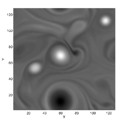
Figure 1: Visualization of the field $-\Delta\Phi$ for the choice of parameters $\lambda=1$, $g=0.1$, $\nu=7\;10^{-6}$, $L=20$, $N=128^{2}$ with no forcing. The field is “smooth” and appears as being isotropic. A few vortices are present. The gray coloring scheme scales from -4.5 (black) to 4.5 (white)

To obtain the “smooth” field depicted in Fig. 1, we carried out simulations with no forcing $(F_{0}=0)$ and a low dissipation. The parameters for this run were $\lambda=1$, $g=0.1$, $\nu=7\;10^{-6}$. Due to this low dissipation the energy may be considered as constant for the length of the simulation. We notice that a few distinct vortices are present. During the evolution a merger between two vortices occurred. There is also an average drift in the y-direction.

II.5.2 Forced Field

To obtain the “forced” field depicted in Fig. 2, we carried out simulations with a strong forcing and dissipation, the parameters for this run were $\lambda=4$, $g=0.1$, $\nu=5\;10^{-5}$, $F_{0}=4$, $k_{0}=6\pm 2$,

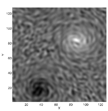
Figure 2: Visualization of the field $-\Delta\Phi$ for the choice of parameters $\lambda=4$, $g=0.1$, $\nu=5\;10^{-5}$, $F_{0}=4$, $k_{0}=6\pm 2$ , $\Delta t=2$. Two big perturbed vortices are present. The gray coloring scheme scales from -1.4 (black) to 1.4 (white)

the phases for the random forcing were updated every $\Delta\tau=2$ time units. The value of $k_{0}$ corresponds to physical scales of $\delta x\sim\frac{2\pi}{k_{0}}\approx 1$. With this choice of parameters the system consists of two perturbed vortices. An average drift in the y-direction is also noticeable.

II.5.3 Anisotropic Field

To obtain the “anisotropic ” field depicted in Fig. 3, we carried out simulations with some forcing and a high value for $g$. The parameters for this run were $\lambda=0.125$, $g=2$, $\nu=7.5\;10^{-6}$, $F_{0}=1.5$, $k_{0}=12\pm 2$. The value of $k_{0}$ corresponds to physical scales of $\delta x\sim\frac{2\pi}{k_{0}}\approx 0.5$. The phases for the random forcing are updated every $\Delta\tau=2$ time units. In this settings elongated structures as well as a strong drift in the y-direction is present.

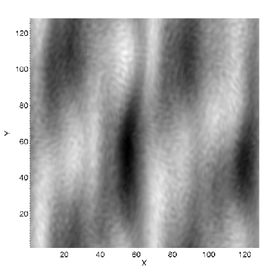
Figure 3: Visualization of the field $-\Delta\Phi$ for the choice of parameters $\lambda=0.125$, $g=2$, $\nu=7.5\;10^{-6}$, $F_{0}=1.5$, $k_{0}=12\pm 2$, $\Delta t=2$. Elongated structures in the y-direction are present, marking a strong anisotropy. The gray coloring scheme scales from -1.6 (black) to 1.6 (white)

III Transport properties

III.1 Definitions

Unfortunately the deterministic description of the motion of a passive particle in a chaotic region is impossible. Local instabilities produce exponential divergence of trajectories. Thus even an idealized numerical experiment is non-deterministic, as round-off errors are creeping slowly but steadily from the smallest to the observable scale. The long-time behavior of tracer trajectories is then necessarily studied by using a probabilistic approach. In the absence of long-term correlations, the kinetic description, which uses the Fokker-Plank-Kolmogorov equation, leads to Gaussian statistics. Yet if a phenomenon with associated long time correlations occurs, profound changes in the kinetics can be induced. These memory effects sometimes result in the modification of the diffusion coefficient in the FPK equation Chirikov79 ; Rechester80 . But often their influence is more profound zaslavsky93 ; DcN98 ; Castiglione99 ; Kuznetsov2000 ; LKZ01 ; LZ02 , and leads to non-Gaussian statistics, and for instance to a non-diffusive behavior of the particle displacement variance:

$$\langle(s-\langle s\rangle)^{2}\rangle\sim t^{\mu}\>,$$ (13)

where $\langle\cdots\rangle$ stands for ensemble averaging. Within this probabilistic approach, the main observables in order to characterize transport properties will be moments of the distributions:

$$M_{q}(t)=\langle|s(t)-\langle s(t)\rangle|^{q}\rangle\>,$$ (14)

where $q$ denotes the moment order. The finiteness of velocity and of time in our simulations implies that all moments are finite and that a power law behavior is expected

$$M_{q}\sim D_{q}t^{\mu(q)}\>.$$ (15)

with, generally, $\mu(q)\neq q/2$ as would be expected for normal diffusion. The nonlinear dependence of $\mu(q)$ is a signature of the multifractality of the transport, while its linear dependence reflects a fractal situation Castiglione99 ; Andersen2000 ; Ferrari01 . In the fractal situation all of the moments can be described by a single self-similar exponent $\nu$

$$\mu(q)=\nu\cdot q\>,$$ (16)

whereas the case when $\mu(q)$ is nonlinear

$$\nu(q)\equiv\frac{\mu(q)}{q}\neq const\>,$$ (17)

transport is multifractal. This distinction is important since in the weak case the PDF evolves in a self-similar way:

$$P(s,t)=t^{-\nu}f(\xi),\hskip 28.45274pt\xi\equiv t^{-\nu}(s-\langle s\rangle)$$ (18)

while a non-constant $\nu(q)$ in (17) precludes such self-similarity (see the discussions in Kuznetsov2000 ; LKZ01 for details about the non self-similar behavior).

In order to characterize transport, we focus on the arc length $s(t)$ of the path traveled by an individual tracer up to a time $t$,

$$s_{i}(t)=\int_{0}^{t}v_{i}(t^{\prime})dt^{\prime}\>,$$ (19)

where $v_{i}(t^{\prime})$ is the absolute speed of the particle $i$ at time $t^{\prime}$. This choice is motivated by the fact that in order to consider mixing properties from the dynamical principles it is important to consider the trajectories within the phase space. However, for the system of passive particles the phase space is formally “identical” to the physical space where particles evolve (see Eq.9). Another important feature of the arc length is that it is independent of the coordinate system and as such we can expect to infer intrinsic properties of the dynamics. Moreover, expression (19) implies that $s_{i}(t)$ reflects the history up to time $t$ of the speed $v_{i}$. Since the velocities are bounded the observations described further on of anomalous transport behavior are directly linked to strong memory effects.

III.2 Particle Transport

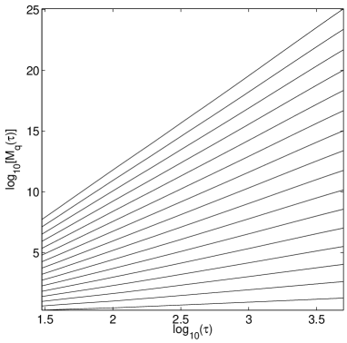
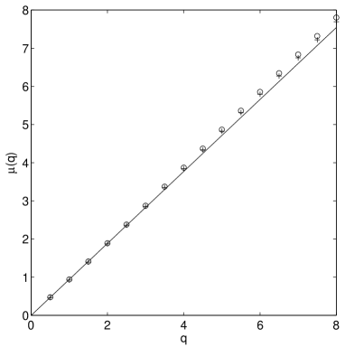
Figure 4: Top: Moments of distribution of the arc length $M_{q}(\tau)=\langle|s(\tau)-\langle s(\tau)\rangle|^{q}\rangle$ versus time of tracers evolving in the smooth field for $q=1/2,\>1,\>3/2,\cdots 8$. The behavior $M_{q}(\tau)\sim\tau^{\mu(q)}$ is confirmed. Bottom: Characteristic exponent versus moment order, $q$ vs $\mu(q)$, with $\mu(2)=1.87$. o and + symbols refer respectively to computations made using 512 and 256 particles. The solid line corresponds to $\mu(q)=\mu(1)q$ expected for self-similar behavior. Transport is super-diffusive and multifractal.

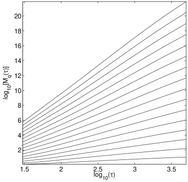
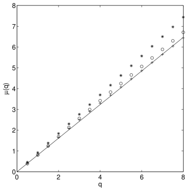
Figure 5: Top: Moments of distribution of the arc length $M_{q}(\tau)=\langle|s(\tau)-\langle s(\tau)\rangle|^{q}\rangle$ versus time of tracers evolving in the forced field for $q=1/2,\>1,\>3/2,\cdots 8$. The behavior $M_{q}(\tau)\sim\tau^{\mu(q)}$ is confirmed. Bottom: Characteristic exponent versus moment order, $q$ vs $\mu(q)$, with $\mu(2)=1.68$. One can notice a change of slope after $\log_{10}(\tau_{0})=3.3$. The o and + symbols refer respectively to computations made using 512 and 256 particles for $\tau>\tau_{0}$, while the * sign corresponds to $\tau<\tau_{0}$. The solid line corresponds to $\mu(q)=\mu(1)q$ expected for self-similar behavior. Transport is super-diffusive.

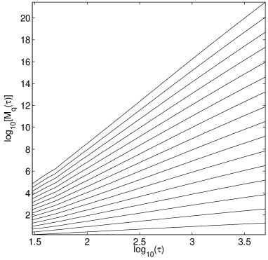
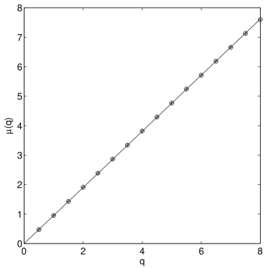
Figure 6: Top: Moments of distribution of the arc length $M_{q}(\tau)=\langle|s(\tau)-\langle s(\tau)\rangle|^{q}\rangle$ versus time of tracers evolving in the anisotropic field for $q=1/2,\>1,\>3/2,\cdots 8$. The behavior $M_{q}(\tau)\sim\tau^{\mu(q)}$ is confirmed. Bottom: Characteristic exponent versus moment order, $q$ vs $\mu(q)$, with $\mu(2)=1.85$. o and + symbols refer respectively to computations made using 512 and 256 particles. The solid line corresponds to $\mu(q)=\mu(1)q$ expected for self-similar behavior. Transport is super-diffusive and single fractal.

We followed the evolution of $512$ passive particles as defined by Eq.(8), and we computed $s_{i}(t)$’s up to a time $\tau=10^{4}$. In order to keep a constant numerical accuracy the increments $\Delta s_{i}(nT)=s_{i}((n+1)T)-s_{i}(nT)$ were recorded for the successive diagnostic times $nT$. This last feature has also the advantage of providing better statistics when computing moments. Indeed since we have chosen stationary regimes for the field, we can assume that transport properties are independent of the initial condition of the field and thus use time-invariance to increase statistics. This time invariance becomes however not useful for times close to $\tau=10^{4}$, and statistics in this region is thus not accurate anymore, also we are not interested in short time behavior. We have therefore considered times $10^{2}<\tau<5.10^{3}$ in order to compute the $\mu(q)$.

In all three considered cases the transport is found to be anomalous and superdiffusive, with a characteristic second order exponent $\mu(2)\approx 1.8$ for all cases. The time behavior of the moments and characteristic exponents for all considered cases are plotted in figures 4, 5 and 6, and a summary is provided in table 2, where we included for comparison the results obtained in Ref. LZ02 for a flow governed by point vortices. The similarity observed for the exponents in these quite different settings of the parameters and regimes of the Charney-Hasegawa-Mima equation as well as the one observed in point vortices, points to a universal behavior for the transport of passive tracers in these two-dimensional flows, which in some sense confirms the validity of the quite general estimation of $\mu\approx 1.5$ proposed in LKZ01 as a value for an universal exponent.

However, conversely to the point vortices case, one can notice from Figs. 4, 5 and 6 that the behavior of characteristic exponent versus moment for the first two cases may correspond more to the multifractal type although the nonlinearity is quite weak, and error bars are quite large. For the third case, transport is more or less simply fractal. This behavior corresponds to simple fractal transport in the anisotropic system,

Table 2: Characteristic second moment exponent for the three different cases studied. Exponents obtained in flows governed by point vortices in Ref. LZ02 are given for comparison.

Point vortices	4 vortices $\mu(2)\approx 1.82$ 16 vortices $\mu(2)\approx 1.77$
Charney-Hasegawa-Mima	Smooth Field $\mu(2)\approx 1.81$ Forced Field $\mu(2)\approx 1.73$ Anisotropic Field $\mu(2)\approx 1.85$

which implies an almost self-similar behavior of the distribution function. In fact as may be illustrated in figure 5, we may expect that with more particles and larger times the multifractal behavior may be more clear, a feature which can also be the case for the third case. When computing characteristic exponents one also has to recall the possibility of log-periodic oscillations Benkadda99 . This phenomenon may also be responsible for the uncertainties on the measured values of the exponents.

All in all these results imply that at least for intermediate times, transport is anomalous and single fractal, which means that transport properties in these systems should be correctly described by a fractional Fokker-Plank-Kolmogorov equation of the type Zaslavsky2002 :

$$\frac{\partial^{\beta}P(s,t)}{\partial t^{\beta}}=\mathcal{D}\frac{\partial^{\alpha}P(s,t)}{\partial|s|^{\alpha}}\>,$$ (20)

with $\mu\approx 2\beta/\alpha$ (see for instance LKZ01 ; Zaslavsky2002 ). For larger time transport may remain single fractal or develop a multifractal behavior in which case a model of transport properties using Eq.(20) may be only approximate. Note that using Eq.(20) to model transport properties implies that a kinetic limit has been performed on particle statistics. In this situation we are dealing with Levy type processes, hence moments higher than two are likely not defined. This particularity is however linked to the kinetic limit, and since we are dealing numerically with a finite number of particles during a finite time, and also since velocities are bounded, moments of particle arc-length distribution are defined, see Zalavsky2000 for a discussion on the matter.

IV Jets

IV.1 Definitions

Tracking the origin of anomalous transport can be fairly well understood when one is able to draw a phase portrait using a Poincare map and for instance to measure Poincare return time to a given region of phase space. The conclusion of this type of analysis will almost certainly lead to the fact that the phenomenon of stickiness on the boundaries of the islands generates strong “memory effects”, as a result of which transport becomes anomalous. However, when dealing with a more complex system, for which the drawing of a phase portrait is not achievable, one has to rely on other techniques.

Figure 7: Tracking of $\epsilon$ coarse-grained regular jet.

In a two dimensional phase-space, the phenomenon of stickiness corresponds often to passive particles remaining for large times in the neighborhood of an island of regular motion. A consequence of this behavior is that sticky zones are regions where particles are trapped, and therefore are regions where particles remain in each others neighborhood for large times. It becomes then natural when dealing with more complex systems for which no phase portrait can easily be drawn, to look for places where passive particles remain in each other’s vicinity for large times. One possibility to capture this feature of the dynamics is to look for its signature by measuring finite time Lyapunov exponents (FTLE), and by isolating within the space of initial conditions, regions of vanishing FTLE’s (see for instance Boatto99 ). This type of approach has however its shortcoming, namely sticky regions are not necessarily smooth from the microscopic point of view, meaning they can be regions of strong chaos that are somehow restricted within an arbitrary small scale, which may be problematic when dealing with FTLE’s. The other possibility is to look directly for chaotic jets LZ02 . These chaotic jets can be understood as moving clusters of particles within a specific domain for which the motion appears as almost regular from a coarse grained perspective. From another point of view, looking for chaotic jets can be understood as a particular case of measurements of space-time complexityAfraimovich03 .

In order to look for jets we proceed as described in the illustration presented in Fig. 7 which provides an easy and intuitive description of the mechanism used to detect jets. To summarize, we consider a reference trajectory $\mathbf{r}(t)$ within the phase space. We then associate to this trajectory a corresponding “coarse grained” equivalent, i.e the union of the balls $\cup B(\mathbf{r}(t),\epsilon)$ of radius $\epsilon$ whose center is the position $\mathbf{r}(t)$. Given an $\epsilon$-coarse grained trajectory, we analyze the behavior of real trajectories starting from within the ball at a given time, and measure the time $\tau$ and length $s$, before the trajectory escapes from the coarse grained trajectory. We then analyze the resulting distributions. This approach has already been used with success when studying numerically the advection of passive tracers in flows governed by point vortices LZ02 . The main difficulty in using this diagnostic follows from the fact that data acquisition is not sampled linearly in time nor space, a point which leads in the present case to some difficulties.

IV.2 Statistical results

In the setting of the evolution of passive tracers within the three considered Charney-Hasegawa-Mima flows, we settled for the following values $\epsilon=10^{-1}$ and $\delta=10^{-3}$. These values are to be compared with the $\epsilon=10^{-2}$ and $\delta=10^{-6}$ considered for point vortex systems in LZ02 .

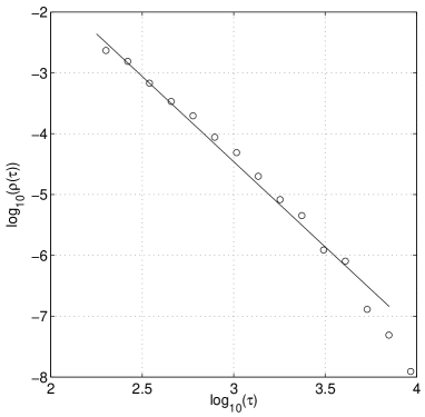
Figure 8: Tail of the distribution of trapping times $\tau$ for the smooth field (Fig. 1). A power-law decay is observed with typical exponent $\rho(\tau)\sim\tau^{-\gamma}$ with $\gamma\approx 2.8\pm 0.1$.

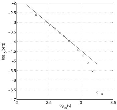
Figure 9: Tail of the distribution of trapping times $\tau$ for the forced field (Fig. 2). A power-law decay is observed with typical exponent $\rho(\tau)\sim\tau^{-\gamma}$ with $\gamma\approx 2.8\pm 0.1$.

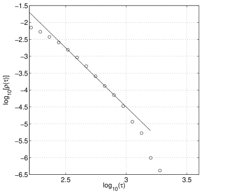
Figure 10: Tail of the distribution of trapping times $\tau$ for the anisotropic field (Fig. 3). A power-law decay is observed with typical exponent $\rho(\tau)\sim\tau^{-\gamma}$ with $\gamma\approx 3.5\pm 0.5$.

This reduction of accessible scales stems from the fact that for the length of our simulations ($\tau=10^{4}$), only a few trajectories are escaping from the jets when we try to use the point vortex values. This leaves us with not enough data to gather realistic statistics. It is important to note that results should not depend much on the value of $\epsilon$ (see the discussion in LZ02 ), as long as its value does not cross a characteristic scale in the system. For instance in the point vortex systems, cores surrounding vortices had a radius of order $\sim 0.1$, or here in the forced systems, the characteristic wavelength corresponds to scales of order $\sim 1$. Moreover in order to infer some possible fractal structure of the jet, we are constrained to consider the largest possible $\epsilon$ once $\delta$ has been fixed. Here the choice made for $\delta$ was the smallest we could make in order to gather enough statistics, although these may not be sufficient for the anisotropic case. We also tried to keep at least two orders of magnitude between $\epsilon$ and $\delta$, to infer eventual fractal properties.

With the present choice of parameters we were able for gather about $15000$ events for each of the three cases. We followed $256$ reference trajectories for a time $\tau=10^{4}$ during which the behavior of two nearby tracers was checked. We call a reference trajectory the trajectory of a given passive tracer which evolves freely, we then put randomly at a distance $\delta$ of this tracer a second (or more) tracer which was called a ghost in LZ02 . We then let these tracer evolve until the distance $\epsilon$ is reached. Then the ghost is removed and time interval $\Delta\tau$ and travelled length $\Delta s$ are recorded. A new ghost is assigned to the reference trajectory and so on. We of course expect that the portion we compute of reference trajectory ($\tau=10^{4}$) is sufficiently ergodic in the accessible phase space.

We were then able to obtain the trapping time distributions $\rho(\tau)$ described in Figs. 8, 9 and 10. The characteristic exponent $\rho(\tau)\sim\tau^{-\gamma}$ for trapping times observed in two out of the three systems is typically $\gamma\approx 2.8$. For these cases we therefore obtain good agreement with the

$$\gamma\approx\mu(2)+1\>,$$ (21)

relation which links the transport exponent $\mu$ to the characteristic trapping time exponent. The law (21) can be linked to the fractional transport equation (20). One can link the $\gamma$ exponent to the $\beta$ exponent as follows $\beta=\gamma-1$ , and $\mu=2\beta/\alpha$ (see LKZ01 ; LZ02 and references therein). $\alpha$ being linked to the spatial fractal properties, the equation (21) is valid when $\alpha\sim 2$. One can also notice in Fig.s. 8, 9 that the law $\rho(\tau)\sim\tau^{-\gamma}$ applies typically for times up to $\tau\sim 1000$ or a little more. This behavior can be expected as we are following a finite number of reference trajectories ($256$) during a finite time ($\tau_{max}=10^{4}$). In order to potentially obtain a broader range of applicability one, would have to increase the value of $\tau_{max}$ to at least $10^{5}$. This is unfortunately beyond our computing resources. Note also, that due to the inverse cascade there is an accumulation of energy at large scales, such that the driving field may not always be considered to have reached a stationary state if we decided to increase simulation length. In order get better statistics, one also has to be careful in not adding to many particles instead of increasing time. Indeed the limits $N\rightarrow\infty$ and $\tau\rightarrow\infty$ are most likely not commuting in these anomalous regimes where rare events related to memory effects are important.

In fact the law (21) also applies in the anisotropic field for small trapping times, but o. verth whome range it is clear in Fig. 10 that no scaling law really emerge. When comparing with the two other cases, we may find two possible reason for this failure. First, we can notice that in this configuration of the field the energy and enstrophy are quite low, implying weak nonlinear effects. It may thus take more time to fill the tail of the trapping time distribution. Second, another peculiarity of the anisotropic case is the the fact pointed out in Basu03 ; Basu_03 : in the anisotropic case, the conservation of the generalized vorticity $\Omega=\Phi-\lambda\Delta\Phi+gx\>,$ by the evolution of the Hasegawa-Mima equation (1) implies necessarily that for strong values of $g$ the motion along the $x-$direction is bounded. Hence in this situation the motion of passive tracers is quasi one dimensional. In this setting it is likely that the hidden fractal properties in the system may differ than for a two-dimensional systems, especially regarding the derivation of the laws linking $\beta$, $\gamma$ and $\alpha$. In these regards, the fact that the law (21) is valid for small times up to a time $\tau_{c}$ may just be a simple consequence of the fact that for $\tau<\tau_{c}$, the passive tracers have not yet reached the boundaries imposed by $g$ and a spatially two dimensional behavior is still accurate. At this point it is important to recall that we have periodic boundary conditions. The constraint imposed by the conservation of $\Omega$ is thus not as important for small values of $g$ corresponding to the first two cases.

The rarity of events with smaller values of $\delta$ indicates that the trajectories of tracers are relatively regular when one considers small scales, which implies the possibility of vanishing Lyapunov exponents. Hence, following the definitions given in LZ02 :

$$\sigma_{L} = \frac{1}{\Delta t}\ln\frac{\epsilon}{\delta}\>,$$ (22)

$$\sigma_{D} = \frac{1}{\Delta s}\ln\frac{\epsilon}{\delta}\>,$$ (23)

we compute the distribution of Lyapunov exponents $\sigma_{D}$ obtained from the smooth case data in Fig. 11

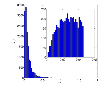
Figure 11: Unnormalized Distribution of Lyapunov exponents $\sigma_{D}$, see Eq. (23). An accumulation towards zero is observed. The zoom near small regions reveals an actual decrease for $\sigma_{D}<0.02$, such behavior is expected as data is bounded by finite speed and finite time.

, where one can directly see an accumulation towards zero of the distribution. The zoom in Fig. 11 shows an actual decrease for $\sigma_{D}<0.02$. This behavior is expected as we only have finite speeds in the system and simulations are carried for a finite time. For instance $\sigma_{D}<0.02$ corresponds to an average trapping time $t_{a}=1100$. This accumulation of exponents toward zero is quite important as it is a strong evidence of memory effects. The system does not display universal hyperbolic properties, and thus transport modeling using this as a hypothesis are probably doomed. This also shows the relevance of the notion of weak chaos and weak mixing properties, and therefore the necessity of considering simple models such as the billiard considered in Zaslav2001 . Indeed these provide good insights on how the presence of quasi zero Lyapunov exponents does not necessary mean the system is regular, but that complexity is not growing as fast as expected Afraimovich03 .

IV.3 Localization and structure of jets

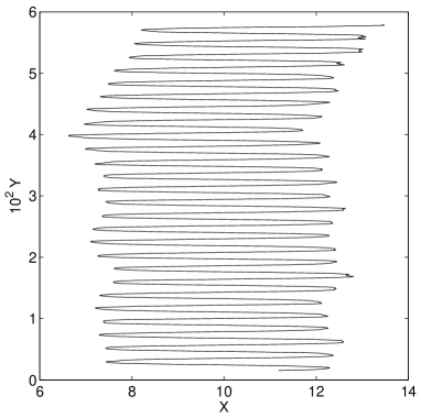
Figure 12: Localization of a long lived jet in the “Forced Field” (cf Fig. 2). The jet is bouncing back and forth between the two perturbed vortices

Due to the shape of the finite size Lyapunov exponent distributions observed, it is also possible to track and localize jets which are responsible for the anomalous behavior. Indeed, these exponents are monotonically decreasing. Hence we can define a threshold beyond which the jet can be considered “regular”. We can track the reference trajectory afterwards in order to localize regions responsible for anomalous behavior. In Fig. 12 we show the localization of a jet for which the trapping time of nearby tracers is found to be $\approx 1000$, in the case of the forced field (cf Fig. 2). The jet is bouncing back and forth between the two perturbed vortices.

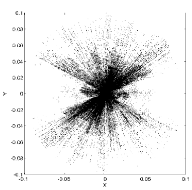
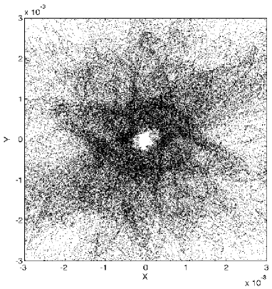
Figure 13: Relative position of test particles for the long lived jet depicted in Fig. 12 (top). Zoom (bottom), test particles reach distances $<10^{-4}$ to the reference trajectory.

The procedure to detect a jet is quite simple, we chose a reference trajectory and start to compute trapping times of ghosts. When we notice that a ghost has not escaped for a while (we choose $\tau>200$ for this jet), we start recording the positions of the reference tracer. We also reset the ghosts and add many more in order to track the “structure” of the jet, and record their positions as well. When one of the ghosts leave the jet, we measure the actual trapping time. If it appears long enough (here we chose $\tau>1000$), we stop, else we reset everything and wait until the reference trajectories detect a new potential jet. The advantage of this method is that we have no a priori information on the jet location. For instance the jet depicted in Fig.  12, was not anticipated, as we expected more a trapping within a vortex or in its neighborhood. We may notice however that by using this method of detection we miss the first portion of the jet. Note also that by localizing jets, we are able to detect regions responsible for anomalous behavior of transport properties. It therefore may therefore give a good clue on where and how to act on a system, if one wants to reduce or eliminate this anomaly.

Once a jet is located, one can infer the behavior of the test tracers with respect to the reference trajectory. In order to get Fig. 13, 256 test particles were initialized on a circle around a reference particle whose trajectory was trapped in the long lived jet localized in Fig. 12, and the relative positions of the test particles were plotted during the life of the jet. One notices a “star” like shape of the figure, this phenomenon is a consequence of multiple stretching and squeezing of the circle of particles, which one can observe while looking dynamically at the evolution of the circle. One also can notice that ghosts which initially are localized at a distance $\delta=10^{-3}$ from the reference tracer, can find themselves much closer to the test particles close to $10^{-4}$ in Fig. 13. This implies that we do not expect that the value of the trapping time exponent $\gamma$ is strongly dependent on the initial choice of $\delta$. Note also that the behavior portrayed in Fig. 13 seems to indicate that chaos is present at these scales, thus contrary to our physical intuition the relative motion within the jet is not regular. However despite this fact, the chaotic behavior of trajectories is trapped within a given small scale for a long time, which in the end gives rise to a regular non-diffusive trajectory from a coarse grained perspective. This trapping phenomena is also illustrated by the apparently “quantified” maximum radii seen on the star shape displayed in Fig. 13. We may thus speculate that these radii correspond to actual successive barriers which are restricting chaos within a small scale. Note also that the chaotic behavior within the jet may have induced numerical computations of strong values for finite time Lyapunov exponents. In this situation relying on these exponents would have meant that jets which are responsible for anomalous transport may go unnoticed.

V Conclusion

In this paper we have investigated the dynamical and statistical properties of passive particle advection in different configurations of Charney-Hasegawa-Mima flows. The goal of the work was to consider transport properties of these systems while putting in perspective the results obtained for point vortex flows. In this sense it was a step further in providing qualitative insights on general transport properties of two-dimensional flows. The transport properties of all the considered cases are found to be anomalous with characteristic exponent $\mu\sim 1.75-1.8$. These values are also quantitatively comparable to the results obtained for point vortex flows.

In order to analyze the origin of the anomalous transport properties, passive tracer motion is analyzed by measuring the mutual relative evolution of two nearby tracers, i.e by looking for chaotic jets LZ02 . The jets can be understood as moving clusters of particles within a specific domain where the motion is almost regular from a coarse grained perspective, inducing memory effects and long time-correlations. The distribution of trapping times in the jets shows a power-law tail whose characteristic exponent is in very good agreement with the law $\gamma=\mu+1$ linking the transport exponent $\mu$ to the trapping time exponent $\gamma$. This agreement is a good signature that the origin of anomalous transport in these system is intimately related to the existence of jets in the sense described previously. The localization of jets in the system can be done, and it is shown that jets are not necessarily located around a coherent structure as was the case for point vortex flows, but that they can manifest themselves by a trajectory bouncing back and forth between 2 structures. Moreover when analyzing the “structure” of the jet, it is shown that the trajectory of individual tracers are likely chaotic within the jet, but that this chaotic behavior is for long times restricted within a given small scale, giving rise to the regular non-diffusive structure.

- [1] M. F. Schlesinger, G. M. Zaslavasky, and J. Klafter. Nature, 363:31, 1993.
- [2] B. A. Carreras, V. E. Lynch, L. Garcia, M. Edelman, and G. M. Zaslavsky. Topological instability along filamented invariant surfaces. Chaos, 13(4):1175, 2003.
- [3] S. V. Annibaldi, G. Manfredi, R. O. Dendy, and L. O’C. Drury. Evidence for strange kinetics in hasegawa-mima turbulent transport. Plasma Phys. Control. Fusion, 42:L13–L22, 2000.
- [4] D. del Castillo-Negrete, B. A. Carreras, and V. E. Lynch. Fractional diffusion in plasma turbulence. Phys. Plasmas, 11(8):3584, 2004.
- [5] V. Grandgirard, O. Agullo, S. Benkadda, B. Biehler, X. Garbet, P. Ghendrih, and Y. Sarazin. Impurity transport in flux driven models of edge turbulence. Proceedings of the Varenna conférence, "Theory of Fusion Plasmas", Editors J.W. Connor, O. Sauter and E. Sindoni, pages pages 427 – 432, 2000.
- [6] G. M. Zaslavsky. Chaos, fractional kinetics, and anomalous transport. Phys. Rep., 371:641, 2002.
- [7] L. Kuznetsov and G. M. Zaslavsky. Passive particle transport in three-vortex flow. Phys. Rev. E., 61:3777, 2000.
- [8] X. Leoncini, L. Kuznetsov, and G. M. Zaslavsky. Chaotic advection near 3-vortex collapse. Phys. Rev.E, 63(036224), 2001.
- [9] X. Leoncini and G. M. Zaslavsky. Jets, stickiness and anomalous transport. Phys. Rev. E, 65(046216), 2002.
- [10] V. V. Afanasiev, R. Z. Sagdeev, and G. M. Zaslavsky. Chaotic jets with multifractal space-time random walk. Chaos, 1:143, 1991.
- [11] Xavier Leoncini and George M. Zaslavsky. Chaotic jets. Communications in Nonlinear Science and Numerical Simulation, 8:265–271, 2003.
- [12] V. Afraimovich and G. M. Zaslavsky. Space-time complexity in hamiltonian dynamics. CHAOS, 13(2):519–532, 2003.
- [13] A. Hasegawa. Adv. Phys., 34, 1981.
- [14] J. Pedlosky. Geophysical Fluid Dynamics. Springer-Verlag, New-York, 1987.
- [15] S. V. Annibaldi, G. Manfredi, and R. O. Dendy. Non-gaussian transport in strong plasma turbulence. Phys. Plasmas, 9(3):791, 2002.
- [16] V. Naulin, A. H. Nielsen, and J. Juul Rasmussen. Dispersion of ideal particles in a two dimensional model of electrostatic turbulence. Phys. Plasmas, 6(12):4575, 1999.
- [17] R. Dickman. Fractal rain distributions and chaotic advection. Brazilian Journal of Physics, 34:337, 2004.
- [18] F. Dupont, R. I. McLachlan, and V. Zeitlin. On possible mechanism of anomalous diffusion by rossby waves. Phys. Fluids, 10(12):3185, 1998.
- [19] J. Sukhatme. Lagragian velocity correlations and absolute dispersion in the midlatitude troposphere. J. Atmos. Sci, arXiv:physics/0410130, submitted, 2004.
- [20] P. Beyer and S. Benkadda. Advection of passive particles in the kolmogorov flow. Chaos, 11(4):774, 2001.
- [21] O. Agullo and A. Verga. Relaxations towards localized vorticity states in drift plasmas and geostrophic flows. Phys. Rev. E, 69:056318, 2004.
- [22] C.F. Fontán and A. Verga. Dynamics of coherent structures and turbulence of plasma drift waves. Phys. Rev. E, 52:6717, 1995.
- [23] R.I. McLachlan and P. Atela. The accuracy of symplectic integrators. Nonlinearity, 5:541, 1992.
- [24] L. Kuznetsov and G. M. Zaslavsky. Regular and chaotic advection in the flow field of a three-vortex system. Phys. Rev E, 58:7330, 1998.
- [25] A. Laforgia, X. Leoncini, L. Kuznetsov, and G. M. Zaslavsky. Passive tracer dynamics in 4 point-vortex-flow. Eur. Phys. J. B., 20:427, 2001.
- [26] B. V. Chirikov. Universal instability of many-dimensional oscillator systems. Phys. Rep. 52, 52:263, 1979.
- [27] A.B. Rechester and R. White. Calculation of turbulent-diffusion for the chirikov-taylor model. Phys. Rev. Lett., 44:1586, 1980.
- [28] G.M. Zaslavsky, D. Stevens, and H. Weitzner. Self-similar transport in incomplete chaos. Phys. Rev E, 48:1683, 1993.
- [29] D. del Castillo-Negrete. Asymmetric transport and non-gaussian statistics of passive scalars in vortices in shear. Phys. Fluids, 10:576, 1998.
- [30] P. Castiglione, A. Mazzino, P. Mutatore-Ginanneschi, and A. Vulpiani. On strong anomalous diffusion. Physica D, 134:75, 1999.
- [31] K. H. Andersen, P. Castiglione, A. Massino, and A. Vulpiani. Simple stochastic models showing strong anomalous diffusion. Eur. Phys. J. B, 18:447, 2000.
- [32] R. Ferrari, A. J. Manfroi, and W. R. Young. Strong and weakly self-similar diffusion. Physica D, 154:111, 2001.
- [33] S. Benkadda, S. Kassibrakis, R. White, and G. M. Zaslavsky. Reply to "comment on ’self similarity and transport in the standard map’". Phys. Rev. E, 59:3761, 1999.
- [34] G. M. Zaslavsky. Physica A, 288:431, 2000.
- [35] S. Boatto and R. T. Pierrehumbert. Dynamics of a passive tracer in a velocity field of four identical point vortices. J. Fuild Mech., 394:137, 1999.
- [36] R. Basu, T. Jessen, V. Naulin, and J. J. Rasmussen. Turbulent flux and the diffusion of passive tracers in electrostatic turbulence. Phys. Plasmas, 10(7):2696, 2003.
- [37] R. Basu, V. Naulin, and J. J. Rasmussen. Particle diffusion in anisotropic turbulence. Communications in Nonlinear Science and Numerical Simulation, 8:477–492, 2003.
- [38] G. M. Zaslavsky and M. Edelman. Weak mixing and anomalous kinetics along filamented surfaces. Chaos, 11(2):295–305, 2001.