Hopf Bifurcation and Chaos in a Single Inertial Neuron Model with Time Delay

Abstract

A delayed differential equation modelling a single neuron with inertial term is considered in this paper. Hopf bifurcation is studied by using the normal form theory of retarded functional differential equations. When adopting a nonmonotonic activation function, chaotic behavior is observed. Phase plots, waveform plots, and power spectra are presented to confirm the chaoticity.

Keywords: Hopf bifurcation, time delay, neural network, chaos

1 Introduction

In recent years, dynamical characteristics of neural networks have become a focal subject of intensive research studies. Bifurcations and chaotic phenomena have been investigated in various neural networks. For example, chaotic solutions were obtained in a neural network consisting of 26 neurons in [1]. Numerical solutions of differential equations with electronic circuit models of chaotic neural networks were qualitatively studied in [2]. In [3], a chaotic neural network with four neurons was investigated. Chaotic behavior was found in a cellular neural network with three cells in [4]. In [5], chaotic phenomenon in a three-neuron hysteretic Hopfield-type neural network was discussed. In [6], a high-dimensional chaotic neural network under external sinusoidal force was studied. In [7], bifurcation and chaos as well as their control in a system of strongly connected neural oscillators were discussed. In [8, 9], a discrete-time transiently chaotic neural network was studied. The chaotic phenomenon in a neural network learning algorithm was reported in [10]. Moreover, chaotic behaviors of inertial neural networks are studied in [11, 12]. On the other hand, there are extensive literatures studied neural network models with delays. For example, bifurcations and chaotic dynamics of neural networks with discrete and distributed delays were studied in [13-21].

In this paper, the dynamical behaviors of a single delayed neuron model with inertial terms are investigated. The work presented in this paper can be considered as an extension of the works for inertial neural network without delays [11, 12] to the case with delays, or an extension of the work for single neuron without inertial terms [13] to the case with inertial terms.

The paper is organized as follows. The delayed inertial neuron model is described, and the local stability and the existence of Hopf bifurcation is studied in Section 2. In Section 3, the properties of the bifurcating periodic solutions are analyzed based on the normal form theory developed in [22]. To justify the theoretical analysis, a numerical example is given in Section 4. In Section 5, the observed chaotic behavior of the model with a nonmonotonic activation function is reported. Finally, conclusions are drawn in Section 6.

2 Local stability and the existence of Hopf bifurcation

The single inertial neuron with time delay, similar to that in [13] but with an inertial term, is described by

$$\ddot{x}=-a\dot{x}-bx+cf(x-hx(t-\tau))$$ (1)

where constants $a,b,c>0,h\geq 0$, and $\tau>0$ is the time delay. Without loss of generality, assume that the activation function $f(.)$ in the above equation is a nonlinear function and its third-order continuous derivative exists. Define

$$x_{1}(t)\equiv x(t)-hx(t-\tau),\hskip 14.22636ptt\in[-\tau,+\infty)$$

Then, we have

$$\begin{array}[]{rl}\dot{x}_{1}(t)&=x_{2}(t)\\ \dot{x}_{2}(t)&=-ax_{2}(t)-bx_{1}(t)+cf(x_{1}(t))-chf(x_{1}(t-\tau))\end{array}$$ (2)

The phase space is $C:=C([-\tau,0];R^{2})$. Throughout this paper, assume that the following conditions are satisfied:

$$f(0)=0,\,f^{\prime}(0)>0,\,|c(1-h)|<1/f^{\prime}(0)$$

It is clear that (2) has an unique equilibrium (0, 0) under the above condition. It is also easy to see that if there is no delay term in (1), i.e. $h=0$, then the model is asymptotically stable when

$$b-cf^{\prime}(0)>0.$$ (3)

In the following, we estimate the value of $h$ that preserves the system stability under the above condition.

For convenience, we restate here a result of Bellman and Cooke [24, Theorem 13.9].
Lemma 1 [24]: Let $H(z)\equiv(z^{2}+pz+q)e^{z}+r$, where $p$ is real and positive, $q$ is real and nonnegative, and $r$ is real. Denote by $a_{k}\,(k\geq 0)$ the sole root of the equation

$$\mbox{cot}\,a=(a^{2}-q)/ap$$

which lies on the interval $(k\pi,k\pi+\pi)$. Define the natural number $n$ as follows:

1. if $r\geq 0$ and $p^{2}\geq 2q$, $n=1$;

2. if $r\geq 0$ and $p^{2}<2q$, $n$ is the odd integer $k$ for which $a_{k}$ lies closest to $\sqrt{q-p^{2}/2}$;

3. if $r<0$ and $p^{2}\geq 2q$, $n=2$;

4. if $r<0$ and $p^{2}<2q$, $n$ is the even integer $k$ for which $a_{k}$ lies closest to $\sqrt{q-p^{2}/2}$.

Then, a necessary and sufficient condition under which all the roots of $H(z)=0$ lie to the left of the imaginary axis is that

1. $r\geq 0$ and $(r\,\mbox{sin}\,a_{n})/pa_{n}<1$, or

2. $-q<r<0$ and $(r\,\mbox{sin}\,a_{n})/pa_{n}<1$.

Separating the linear and the nonlinear terms, (2) becomes

$$\dot{x}=L(x_{t})+F(x_{t})$$ (4)

where $x_{t}\in C,x_{t}(\theta)=x(t+\theta),-\tau\leq\theta\leq 0$, and $L:C\rightarrow R^{2},\,F:C\rightarrow R^{2}$ are given respectively by

$$\begin{array}[]{rl}L(\varphi)&=\left[\begin{array}[]{c}\varphi_{2}(0)\\ -(b-cf^{\prime}(0))\varphi_{1}(0)-a\varphi_{2}(0)-chf^{\prime}(0)\varphi_{1}(-\tau)\end{array}\right]\\ F(\varphi)&=\left[\begin{array}[]{c}0\\ \frac{cf^{\prime\prime}(0)}{2}\varphi_{1}^{2}(0)+\frac{cf^{\prime\prime\prime}(0)}{6}\varphi_{1}^{3}(0)-\frac{chf^{\prime\prime}(0)}{2}\varphi_{1}^{2}(-\tau)-\frac{chf^{\prime\prime\prime}(0)}{6}\varphi_{1}^{3}(-\tau)+\cdots\end{array}\right]\end{array}$$ (5)

with $\varphi=(\varphi_{1},\varphi_{2})\in C$. Here and throughout this paper, we refer to [25] for notation and classical results on functional differential equations (FDEs), including such as Eq. (4).

The characteristic equation for the linearization of Eq.(4) at (0, 0) is

$$\lambda^{2}+a\lambda+(b-cf^{\prime}(0))+chf^{\prime}(0)e^{-\lambda\tau}=0$$ (6)

Let $s=\lambda\tau$. Then we have

$$[s^{2}+a\tau s+(b-cf^{\prime}(0))\tau^{2}]e^{s}+chf^{\prime}(0)\tau^{2}=0$$ (7)

The fixed point is locally stable if all roots of the above equation have negative real parts [25]. For each $\tau$, we are interested in the maximum value of $h$ such that the system is locally stable.
Theorem 1: Denote by $w_{k}\,(k\geq 0)$ the sole root of the equation

$$\mbox{cot}\,w=[w^{2}-(b-cf^{\prime}(0))\tau^{2}]/a\tau w$$

which lies on the interval $(k\pi,k\pi+\pi)$. Define the nature number $n$ as follows:

1. if $a^{2}\geq 2(b-cf^{\prime}(0))$, $n=1$;

2. if $a^{2}<2(b-cf^{\prime}(0))$, $n$ is the odd $k$ for which $w_{k}$ lies closest to $\sqrt{(b-cf^{\prime}(0))-a^{2}/2}\,\tau$

Then, under condition (3), a necessary and sufficient condition that the solution of (2) is asymptotically stable is that

$$h<\frac{aw_{n}}{cf^{\prime}(0)\tau\mbox{sin}w_{n}}$$

Proof: Since $a>0,\tau>0,f^{\prime}(0)>0,b-cf^{\prime}(0)>0,h\geq 0$, a direct application of Lemma 1 to (7) with $p=a\tau,q=(b-cf^{\prime}(0))\tau^{2}$ and $r=chf^{\prime}(0)\tau^{2}$ proves the claim.

In the following, we study the existence of Hopf bifurcation in Eq. (2) by choosing $h$ as the bifurcation parameter. First, we would like to know when Eq. (6) has purely imaginary roots $\lambda=\pm i\omega_{0}\,(\omega_{0}>0)$ at $h=h_{0}$. If $\lambda=\pm i\omega_{0},\,\omega_{0}>0$, we have

$$\begin{array}[]{rl}chf^{\prime}(0)\mbox{cos}\,\omega_{0}\tau&=\omega_{0}^{2}-(b-cf^{\prime}(0))\\ chf^{\prime}(0)\mbox{sin}\,\omega_{0}\tau&=a\omega_{0}\end{array}$$

The above equations imply that

$$\mbox{cot}\,\omega_{0}\tau=\frac{\omega_{0}^{2}-(b-cf^{\prime}(0))}{a\omega_{0}}\equiv g(\omega_{0})$$

and, consequently,

$$g^{\prime}(\omega)=\frac{\omega^{2}+(b-cf^{\prime}(0))}{a\omega^{2}}>0$$

So, $g(\omega)$ is strictly monotonically increasing on $(0,+\infty)$, with $\lim_{\omega\rightarrow 0}g(\omega)=-\infty$ and $\lim_{\omega\rightarrow+\infty}g(\omega)=+\infty$. Clearly, $g(\omega)$ intersects $\mbox{cot}\,\omega\tau$ only at a point. Hence, $\lambda=\pm i\omega_{0}$ are simple roots of Eq. (6), where $\omega_{0}$ is the unique root of $\mbox{cot}\omega\tau=\frac{\omega^{2}-(b-cf^{\prime}(0))}{a\omega}$, and $h_{0}=\frac{a\omega_{0}}{cf^{\prime}(0)\mbox{sin}\,\omega_{0}\tau}$.

From [26], we know that all the other roots of Eq. (6) have negative real parts. We proceed to calculate $Re[d\lambda/dh]$ at $h=h_{0}$. Differentiating Eq. (6) with respect to $h$ yields

$$\frac{d\lambda}{dh}=\frac{cf^{\prime}(0)e^{-\lambda\tau}}{ch\tau f^{\prime}(0)e^{-\lambda\tau}-2\lambda-a}$$

So, we have

$$\mbox{Re}\left[\frac{d\lambda}{d\,h}\right]_{\lambda=i\omega_{0}\atop h=h_{0}}=\frac{cf^{\prime}(0)[cf^{\prime}(0)h_{0}\tau-a\mbox{cos}\,\omega_{0}\tau+2\omega_{0}\mbox{sin}\,\omega_{0}\tau]}{(ch_{0}\tau f^{\prime}(0)\mbox{cos}\,\omega_{0}\tau-a)^{2}+(ch_{0}\tau f^{\prime}(0)\mbox{sin}\,\omega_{0}\tau+2\omega_{0})^{2}}$$

From the above analysis, we have the following result.
Theorem 2: Under condition (3), if $cf^{\prime}(0)h_{0}\tau-a\mbox{cos}\,\omega_{0}\tau+2\omega_{0}\mbox{sin}\,\omega_{0}\tau\neq 0$, then as $h$ pass through the critical value $h_{0}=\frac{a\omega_{0}}{cf^{\prime}(0)\mbox{sin}\,\omega_{0}\tau}$, there is a Hopf bifurcation of system (1) at its equilibrium (0, 0), where $\omega_{0}$ is the sole root of $\mbox{cot}\,\omega\tau=\frac{\omega^{2}-(b-cf^{\prime}(0))}{a\omega}$.

Remark: Note that if we let $w=\omega_{0}\tau$, then the constant $h_{0}$ in Theorem 2 can be rewritten as $h_{0}=\frac{aw}{cf^{\prime}(0)\tau\mbox{sin}w}$, which is consistent to that in Theorem 1.

3 Direction and stability of bifurcating periodic solutions

In this section, we study the direction and stability of the bifurcating periodic solutions. The method used here is based on the normal form theory developed by Faria and Magalhães [22]. This method computes normal forms for retarded functional differential equations, without computing beforehand the center manifold of the singularity.

As in [21], in the following we assume $f^{\prime\prime}(0)=0,f^{\prime\prime\prime}(0)\neq 0$. Define $\Lambda=\{-i\omega_{0},i\omega_{0}\}$ and introduce the new parameter $\beta=h-h_{0}$. Eq. (4) can be rewritten as

$$\dot{x}=L_{0}(x_{t})+F_{0}(x_{t},\beta)$$ (8)

where

$$\begin{array}[]{rl}L_{0}(\varphi)&=\left[\begin{array}[]{c}\varphi_{2}(0)\\ -(b-cf^{\prime}(0))\varphi_{1}(0)-a\varphi_{2}(0)-ch_{0}f^{\prime}(0)\varphi_{1}(-\tau)\end{array}\right]\\ F_{0}(\varphi)&=\left[\begin{array}[]{c}0\\ -cf^{\prime}(0)\beta\varphi_{1}(-\tau)+\frac{cf^{\prime\prime\prime}(0)}{6}\varphi_{1}^{3}(0)-\frac{cf^{\prime\prime\prime}(0)}{6}(h_{0}+\beta)\varphi_{1}^{3}(-\tau)+\cdots\end{array}\right]\end{array}$$

Following the formal adjoint theory of FDEs [25], let the phase space $C$ be decomposed according to $\Lambda$ as $C=P\bigoplus Q$, where $P$ is the center space for $\dot{x}=L_{0}(x_{t})$, i.e., $P$ is the generalized eigenspace associated with $\Lambda$. Consider the bilinear form $(\cdot,\cdot)$ associated with the linear equation $\dot{x}=L_{0}(x_{t})$ [23]. Let $\Phi$ and $\Psi$ be bases for $P$ and $P^{*}$ associated with the eigenvalues $\pm i\omega_{0}$ of the adjoint equation, respectively, and normalize them so that $(\Phi,\Psi)=I$. In complex coordinates, $\Phi,\Psi$ are written as $2\times 2$ matrices of the form

$$\begin{array}[]{l}\Phi(\theta)=[\phi_{1}(\theta),\phi_{2}(\theta)],\hskip 5.69046pt\phi_{1}(\theta)=e^{i\omega_{0}\theta}v,\hskip 5.69046pt\phi_{2}(\theta)=\overline{\phi_{1}(\theta)},\hskip 5.69046pt-\tau\leq\theta\leq 0,\\ \Psi(s)=\left[\begin{array}[]{c}\psi_{1}(s)\\ \psi_{2}(s)\end{array}\right],\hskip 5.69046pt\psi_{1}(s)=e^{-i\omega_{0}s}u^{T},\hskip 5.69046pt\psi_{2}(s)=\overline{\psi_{1}(s)},\hskip 5.69046pt0\leq s\leq\tau\end{array}$$ (9)

where the bar means complex conjugation, $u^{T}$ is the transpose of $u$, and $u,v$ are vectors in $C^{2}$ such that

$$L_{0}(\phi_{1})=i\omega_{0}v,\hskip 5.69046ptu^{T}L_{0}(e^{i\omega_{0}s}I)=i\omega_{0}u^{T},\hskip 5.69046pt(\psi_{1},\phi_{1})=1.$$ (10)

Note that $\dot{\Phi}=\Phi B$, where $B$ is the diagonal matrix $B=\mbox{diag}(i\omega_{0},-i\omega_{0})$. From (10), we have

$$\begin{array}[]{c}v_{2}=i\omega_{0}v_{1},\hskip 5.69046pt[-(b-cf^{\prime}(0))-ch_{0}f^{\prime}(0)e^{-i\omega_{0}\tau}]v_{1}=(a+i\omega_{0})v_{2},\\ u_{1}=(a+i\omega_{0})u_{2},\hskip 5.69046pt[-(b-cf^{\prime}(0))-ch_{0}f^{\prime}(0)e^{-i\omega_{0}\tau}]u_{2}=i\omega_{0}u_{1},\end{array}$$ (11)

Hence, we can select

$$v=\left[\begin{array}[]{c}v_{1}\\ v_{2}\end{array}\right]=\left[\begin{array}[]{c}1\\ i\omega_{0}\end{array}\right],\hskip 14.22636ptu=\left[\begin{array}[]{c}u_{1}\\ u_{2}\end{array}\right]=u_{1}\left[\begin{array}[]{c}1\\ \frac{1}{a+i\omega_{0}}\end{array}\right]$$ (12)

with

$$u_{1}=\frac{a+i\omega_{0}}{a+2i\omega_{0}-ch_{0}f^{\prime}(0)\tau e^{-i\omega_{0}\tau}}$$

Here and in the following, we refer to [22] for results and explanations of several notations involved. Enlarging the phase space $C$ by considering the space $BC$ and using the decomposition $x_{t}=\Phi z(t)+y_{t},z\in C^{2},y_{t}\in Q^{1}$, we decompose system (8) as

$$\left\{\begin{array}[]{l}\dot{z}=Bz+\Psi(0)F_{0}(\Phi z+y,\beta)\\ \dot{y}=A_{Q^{1}}y+(I-\pi)X_{0}F_{0}(\Phi z+y,\beta)\end{array}\right.$$ (13)

Consider the Taylor formula

$$\Psi(0)F_{0}(\Phi z+y,\beta)=\frac{1}{2}f_{2}^{1}(z,y,\beta)+\frac{1}{6}f_{3}^{1}(z,y,\beta)+h.o.t.$$

where $f_{j}^{1}(z,y,\beta)\,(j=2,3)$ are homogeneous polynomials in $(z,y,\beta)$ of degree $j$ with coefficients in $C^{2}$ and $h.o.t.$ stands for higher order terms. The normal form on the 2-dimensional center manifold of the origin and $\beta=0$ is given by

$$\dot{z}=Bz+\frac{1}{2}g_{2}^{1}(z,0,\beta)+\frac{1}{6}g_{3}^{1}(z,0,\beta)+h.o.t.$$ (14)

where $g_{2}^{1},g_{3}^{1}$ are second and third order terms in $(z,\beta)$, respectively.

Using the notations in [22], we have

$$\frac{1}{2}g_{2}^{1}(z,0,\beta)=\frac{1}{2}\mbox{Proj}_{\mbox{Ker}(M_{2}^{1})}f_{2}^{1}(z,0,\beta)$$

where $\mbox{Proj}_{S}f$ is the projection of $f$ on $S$, and

$$\mbox{Ker}(M_{2}^{1})=\mbox{span}\left\{\left(\begin{array}[]{c}z_{1}\beta\\ 0\end{array}\right),\left(\begin{array}[]{c}0\\ z_{2}\beta\end{array}\right)\right\}$$

After some computation, we obtain

$$\frac{1}{2}g_{2}^{1}(z,0,\beta)=\left[\begin{array}[]{c}A_{1}z_{1}\beta\\ \overline{A_{1}}z_{2}\beta\end{array}\right]$$

with

$$A_{1}=-cf^{\prime}(0)e^{-i\omega_{0}\tau}u_{2}$$

To compute the cubic terms, we first deduce that, after the change of variables that transformed the quadratic terms $f_{2}^{1}(z,y,\beta)$ into $g_{2}^{1}(z,y,\beta)$, the coefficients of the third order terms at $y=0,\beta=0$ are still given by $\frac{1}{6}f_{3}^{1}(z,0,0)$ (because $f^{\prime\prime}(0)=0$, implying $f_{2}^{1}(z,y,0)=0$). This implies that [22]

$$\frac{1}{6}g_{3}^{1}(z,0,\beta)=\frac{1}{6}\mbox{Proj}_{\mbox{Ker}(M_{3}^{1})}f_{3}^{1}(z,0,\beta)$$

where

$$\mbox{Ker}(M_{3}^{1})=\mbox{span}\left\{\left(\begin{array}[]{c}z_{1}^{2}z_{2}\\ 0\end{array}\right),\left(\begin{array}[]{c}z_{1}\beta^{2}\\ 0\end{array}\right),\left(\begin{array}[]{c}0\\ z_{1}z_{2}^{2}\end{array}\right),\left(\begin{array}[]{c}0\\ z_{2}\beta^{2}\end{array}\right)\right\}$$

However, the terms $O(|z|\beta^{2})$ are irrelevant to the determination of the generic Hopf bifurcation. Hence, we write

$$\frac{1}{6}g_{3}^{1}(z,0,\beta)=\frac{1}{6}\mbox{Proj}_{S}f_{3}^{1}(z,0,0)+O(|z|\beta^{2})$$

for

$$S:=\mbox{span}\left\{\left(\begin{array}[]{c}z_{1}^{2}z_{2}\\ 0\end{array}\right),\left(\begin{array}[]{c}0\\ z_{1}z_{2}^{2}\end{array}\right)\right\}$$

Some computations yield

$$\frac{1}{6}g_{3}^{1}(z,0,\beta)=\left[\begin{array}[]{c}A_{2}z_{1}^{2}z_{2}\\ \overline{A_{2}}z_{1}z_{2}^{2}\end{array}\right]+O(|z|\beta^{2})$$

with

$$A_{2}=\frac{cf^{\prime\prime\prime}(0)}{2}(1-h_{0}e^{-i\omega_{0}\tau})u_{2}$$

Thus, we obtain the normal form (14) with the coefficients $A_{1},A_{2}$ given explicitly in terms of the original equation (4), without the need to compute the center manifold beforehand. The normal form (14) can be written in real coordinates $(x,y)$, through the change of variables $z_{1}=x-iy,z_{2}=x+iy$. In polar coordinates $(r,\theta),x=r\mbox{cos}\theta,y=r\mbox{sin}\theta$, this normal form becomes

$$\left\{\begin{array}[]{l}\dot{r}=K_{1}\beta r+K_{2}r^{3}+O(\beta^{2}r+|(r,\beta)|^{4})\\ \dot{\theta}=-\omega_{0}+O(|(r,\beta)|)\end{array}\right.$$ (15)

where $K_{1}:=Re\,A_{1},K_{2}:=Re\,A_{2}$.

We have the following theorem.
Theorem 3: In formula (15), the sign of $K_{1}K_{2}$ determines the direction of the Hopf bifurcation: if $K_{1}K_{2}<0\,(>0)$, then the Hopf bifurcation is supercritical (subcritical) and the bifurcating periodic solutions exist for $h>h_{0}\,(<h_{0})$; the sign of $K_{2}$ determines the stability of the bifurcating periodic orbits: the bifurcating periodic orbits is stable (unstable) if $K_{2}<0\,(>0)$.

4 A numerical example

Consider an example in the form of system (1), with $a=1,\,b=1.1,\,c=1,\,\tau=1,\mbox{ and }f(.)=\mbox{tanh}(.)$. The theoretical analysis in Section 2 leads to

$$\omega_{0}=0.9017,\hskip 28.45274pth_{0}=1.1496$$

It then follows from the results in Section 3 that

$$K_{1}=0.2627,\hskip 28.45274ptK_{2}=-0.3408$$

These calculations prove that the equilibrium (0, 0) is stable when $h\,<\,h_{0}$, as shown by Fig. 1, where $h=1.1$. When $h$ passes through the critical value $h_{0}=1.1496$, the equilibrium losses its stability and a Hopf bifurcation occurs, i.e., a family of periodic solutions bifurcate from the equilibrium. Each individual periodic orbit is stable for $K_{2}<0$. Since $K_{1}K_{2}<0$, the bifurcating periodic solutions exist at least for values of $h$ slightly larger than the critical value. Choosing $h=1.4$, as predicted by the theory, Fig. 2 shows that there is an orbitally stable limit cycle.

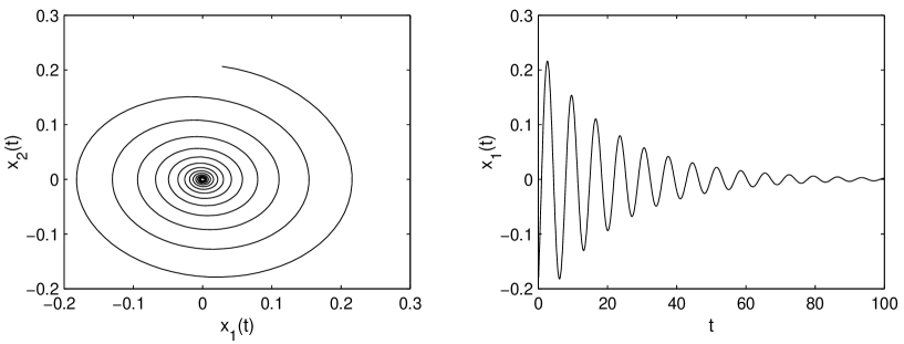
Figure 1: Phase plot and waveform plot for system (1) with $h=1.1$

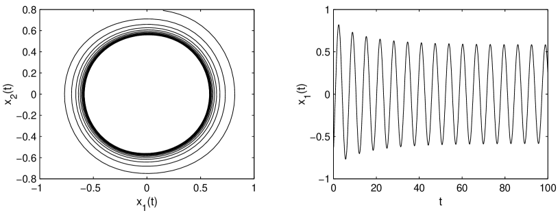
Figure 2: Phase plot and waveform plot for system (1) with $h=1.4$

5 Chaotic behavior

In this section, we study the dynamical behavior of system (1) with the activation function $f(x)=xe^{-x^{2}/2}$ and $a=0.8,b=1,c=5,\tau=5$, and let $h$ be a variable parameter. It is noted that several other parameters have also been examined and shown to exhibit similar dynamical phenomena. Due to limitation of space, those results are not presented here.

When $h<0.65$, the system is stable. When increasing $h$ to $h=0.7$, the system produces a periodic orbit. When $h=0.7$, the phase plot and the waveform plot of $x_{1}(t)$ is shown in Fig. 3. When the value of $h$ passes 0.9, the system becomes chaotic. In Fig. 4, we show the phase plot when $h=1.0$, and in Fig. 5 we show the waveform of $x_{1}(t)$ and the power spectrum plots when $h=1.0$. When $h=5.0$, the phase plot and the waveform of $x_{1}(t)$, and the power spectrum plots, are shown in Fig. 6 and Fig. 7, respectively. From these figures, we can see that the system is also chaotic, but it is different from the case of $h=1.0$.

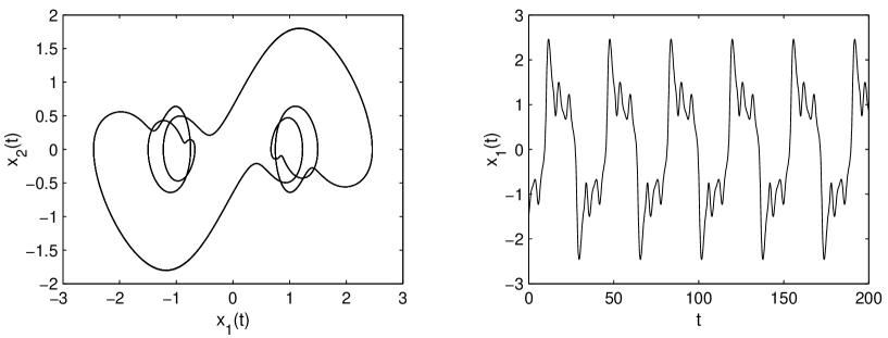
Figure 3: Phase plot and waveform plot when $h=0.7$

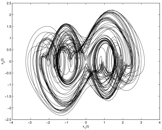
Figure 4: Phase plot when $h=1.0$

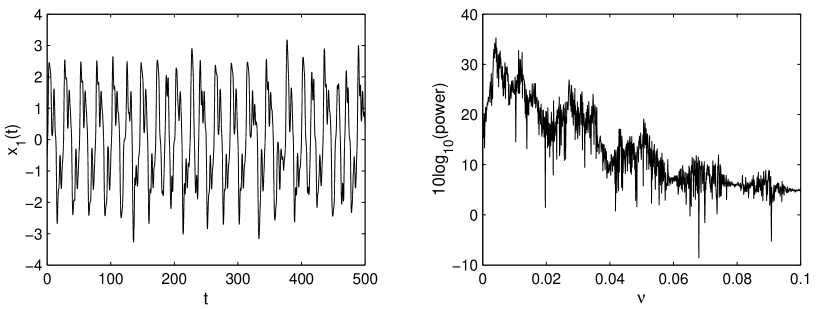
Figure 5: Waveform and power spectrum plots when $h=1.0$

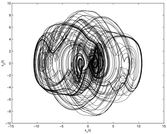
Figure 6: Phase plot when $h=5.0$

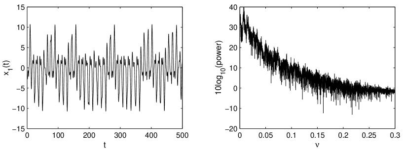
Figure 7: Waveform and power spectrum plots when $h=5.0$

6 Conclusions

A single delayed neuron model with inertial term has been investigated in this paper. Hopf bifurcation is studied by using the normal form theory of retarded FDEs, in which the coefficients of the normal form are obtained in terms of the original delayed equation directly, without the need to compute the center manifold beforehand, which simplifies the computation procedure. With a nonmonotonic activation function, chaotic behavior has also been observed in this system.

References

- [1] K.E. Kurten, J.W. Clark, “Chaos in neural systems”, Physics Letters A, Vol.144, No.7, pp.413-418, 1986.
- [2] T.B. Kepler, S. Datt, R.B. Meyer, L.F. Abbott, “Chaos in a neural network circuit”, Physica D, Vol.46, No.3, pp.449-457, 1990.
- [3] P.K. Das II, W.C. Schieve, Z.J. Zeng, “Chaos in an effective four-neuron neural network”, Physics Letters A, Vol.161, No.1, pp.60-66, 1991.
- [4] F. Zou, J.A. Nossek, “Bifurcation and chaos in cellular neural network”, IEEE Trans. CAS, Vol.40, pp.166-172, 1993.
- [5] C. Li, J. Yu, X. Liao, “Chaos in a three-neuron hysteresis Hopfield-type neural network”, Physics Letters A, Vol.285, pp.368-372, 2001.
- [6] V.E. Bondarenko, “High-dimensional chaotic neural network under external sinusoidal force”, Physics Letters A, Vol.236, pp.513-519, 1997.
- [7] T. Ueta, G. Chen, “Chaos and bifurcation in coupled networks and their control”, in Controlling Chaos and Bifurcations in Engineering Systems, G. Chen (ed.), CRC Press, Boca Raton, 2000, pp.581-601.
- [8] L. Chen, K. Aihara, “Chaotic simulated annealing by a neural network model with transient chaos”, Neural Networks, Vol.8, No.6, pp.915-930, 1995.
- [9] L. Chen, K. Aihara, “Strange attractors in chaotic neural networks”, IEEE Trans. CAS-I, Vol.47, No.10, pp.1455-1468, 2001.
- [10] C. Li, X. Liao, J. Yu, “Generating chaos by Oja’s rule”, Neurocomputing, Vol.55, No.3-4, pp.731-738, 2003.
- [11] K. L. Babcock, R. M. Westervelt, “Dynamics of simple electronic neural networks”, Physica D, Vol. 28, pp. 305-316, 1987.
- [12] D.W. Wheeler, W.C. Schieve, “Stability and chaos in an inertial two-neuron system”, Physica D, Vol.105, pp.267-284, 1997.
- [13] X. Liao, K.-W. Wong, C.-S. Leung, Z. Wu, “Hopf bifurcation and chaos in a single delayed neuron equation with non-monotonic activation function”, Chaos, Solitons and Fractals, Vol.12, pp.1535-1547, 2001.
- [14] X. Liao, Z. Wu, J. Yu, “Stability switches and bifurcation analysis of a neural network with continuously delay”, IEEE Trans. SMC-A, Vol. 29, pp.692-696, 1999.
- [15] X. Liao, K.-W. Wong, Z. Wu, “Bifurcation analysis on a two-neuron system with distributed delays”, Physica D, Vol. 149, pp.123-141, 2001.
- [16] M. Gilli, “Strange attractors in delayed cellular neural networks”, IEEE Trans. CAS, Vol.40, pp.849-853, 1993.
- [17] J. Wei, S. Ruan, “Stability and bifurcation in a neural network model with two delays”, Physica D, Vol. 130, pp.255-272, 1999.
- [18] S. Ruan, J. Wei, “Periodic solutions of planar systems with two delays”, Proc. Roy. Soc. Edingburgh Sect. A, Vol. 129, pp.1017-1032, 1999.
- [19] L. Olien, J. Bélair, “Bifurcations, stability, and monotonicity properties of a delayed neural network model”, Physica D, Vol. 102, pp. 349-363, 1997.
- [20] K. Gopalsamy, I. Leung, “Dealy induced periodicity in a neural netlet of exitation and inhibition”, Physica D, Vol. 89, pp.395-426, 1996.
- [21] T. Faria, “On a planar system modelling a neuron network with memory”, Journal of Diff. Equ., Vol. 168, pp.129-149, 2000.
- [22] T. Faria, L. T. Magalhães, “Normal forms for retarded functional differential equations with parameters and applications to Hopf bifurcation”, Journal of Diff. Equ., Vol. 122, pp.181-200, 1995.
- [23] T. Faria, L. T. Magalhães, “Normal forms for retarded functional differential equations and applications to Bogdanov-Takens singularity”, Journal of Diff. Equ., Vol. 122, pp.201-224, 1995.
- [24] R. Bellman, K. L. Cooke, Differential-Difference Equations, Academic Press, New York, 1963.
- [25] J. K. Hale, S. M. Verduyn Lunel, Introduction to Functional Differential Equations, Springer-Verlag, New York, 1993.
- [26] K. L. Cooke, Z. Grossman, “Discrete delay, distributed delay and stability switches”, J. Math. Anal. Appl., Vol.86, pp.592-627, 1982.