Hopf Bifurcation and Chaos in Tabu Learning Neuron Models

Abstract

In this paper, we consider the nonlinear dynamical behaviors of some tabu leaning neuron models. We first consider a tabu learning single neuron model. By choosing the memory decay rate as a bifurcation parameter, we prove that Hopf bifurcation occurs in the neuron. The stability of the bifurcating periodic solutions and the direction of the Hopf bifurcation are determined by applying the normal form theory. We give a numerical example to verify the theoretical analysis. Then, we demonstrate the chaotic behavior in such a neuron with sinusoidal external input, via computer simulations. Finally, we study the chaotic behaviors in tabu learning two-neuron models, with linear and quadratic proximity functions respectively.

Keywords: Tabu learning, neural network, Hopf bifurcation, chaos

1 Introduction

Neurons as the fundamental elements of the brain can generate complex dynamical behaviors. The studies of nonlinear dynamics in both biological and artificial neural network models are very important in that, on the one hand, the studies may provide explanations for the rich dynamics including oscillations and chaos in biological neural networks, and on the other hand, if we understand more about the dynamical behaviors of various neural networks then we can design some control methods to achieve desirable system behaviors in artificial neural networks.

In recent years, dynamical characteristics of various neural networks have become a focal subject of intensive research studies. Bifurcation and chaos have been identified and investigated in many kinds of neural networks. For example, chaotic solutions were obtained in [Kurten & Clark, 1986], from a neural network consisting of 26 neurons. In [Babcock & Westervelt, 1987], a two-neuron model was studied, with or without time delays. Numerical solutions of differential equations with electronic circuit models of chaotic neural networks were qualitatively compared in [Kepler et al., 1990]. In [Das II et al., 1991], a chaotic neural network with four neurons was investigated, and chaotic behavior was found in [Zou & Nossek, 1993] from a cellular neural network with three cells. In [Li et al., 2001], we also presented some findings of chaotic phenomenon in a three-neuron hysteretic Hopfield-type neural network. In [Bondarenko, 1997], a high-dimensional chaotic neural network under external sinusoidal force was studied. In [Ueta & Chen, 2001], bifurcation and chaos as well as their control in a system of strongly connected neural oscillators were discussed. In [Das et al., 2002], chaos in a three-dimensional general neural network model was investigated. In [Olien & Belair, 1997; Wei & Ruan, 1999; Gopalsamy et al., 1998; Liao et al., 1999; Liao et al., 2001; Liao et al., 2001; Gilli, 1993; Lu, 2002], the bifurcation and chaotic behaviors of various delayed neural networks were studied. Moreover, the chaotic phenomenon in a neural-network-based learning algorithm was reported in [Li et al., 2003].

Tabu learning [Beyer & Ogier, 1991] applies the concept of tabu search [Glover, 1989; Glover, 1990] to neural networks for solving optimization problems. By continuously increasing the energy surface in a neighborhood of the current network state, it penalizes those states that have already been visited. This enables the state trajectory to climb out of local minima while tending toward those areas that have not yet been visited, thus performing an efficient search through the problem’s solution space. Note that, unlike most existing neural-network-based methods for optimization, the goal of the tabu learning method is not to force the network state to converge to an optimal or nearly optimal solution, but rather, the network conducts an efficient search through the solution space. Knowing this, it is very natural for one to ask what the state trajectory of the tabu learning neural network is like? In the present paper, the aim is to provide an answer to this question by studying the dynamical behaviors of the tabu learning neural network.

More precisely, this paper investigates the nonlinear dynamical behaviors of a tabu leaning single neuron model and of two two-neuron models, respectively. By choosing the memory decay rate as a bifurcation parameter, it is proved that Hopf bifurcation occurs in the tabu leaning single neuron model. The stability of the bifurcating periodic solutions and the direction of the Hopf bifurcation are then determined by applying the normal form theory. Chaotic behavior of such a neuron with small sinusoidal external input is also demonstrated by computer simulations. To that end, the chaotic behaviors in tabu learning two-neuron models with linear and quadratic proximity functions, respectively, are studied by means of computer simulations.

The paper is organized as follows. The tabu learning neural network is first described in Section 2. In Section 3, the Hopf bifurcation of a single neuron model is studied. In Section 4, the observed chaotic behavior of the single neuron model is described. In Section 5, the dynamical behaviors of a two-neuron model with a linear proximity function are studied. And, in Section 6, the dynamical behaviors of a two-neuron model with a quadratic proximity function are investigated. Finally, conclusions are drawn in Section 7.

2 Tabu learning neural network

The common problem of minimizing an objective function in many optimization schemes by using the Hopfield-type neural networks of the form

$$C_{i}\dot{u}_{i}=-\frac{1}{R_{i}}u_{i}+\sum_{j}T_{ij}V_{j}+I_{i}$$ (1)

can be translated into minimizing the following energy function:

$$E_{0}=-\frac{1}{2}\sum_{i}\sum_{j}T_{ij}V_{i}V_{j}-\sum_{i}I_{i}V_{i}+\sum_{i}\frac{1}{R_{i}}\int_{0}^{V_{i}}f^{-1}(s)\,ds$$ (2)

where $V_{i}=f(u_{i})$, $f(\cdot)$ is the activation function, $u_{i}$ is the state of neuron $i$, $C_{i}$ and $R_{i}$ are positive constants, $T_{ij}$ represents the strength of the connection from neuron $j$ to neuron $i$, and $I_{i}$ represents the input current to neuron $i$.

In the tabu leaning method, the energy surface $E_{0}$ is continuously increasing in a neighborhood of the current state. At time $t$, the energy surface is given by

$$E_{t}=E_{0}+F_{t}(V)$$ (3)

with

$$F_{t}(V)=\beta\int_{0}^{t}e^{\alpha(s-t)}P(V,V(s))\,ds$$

where $\alpha$ and $\beta$ are positive constants and $P(V,W)$ is a measure of the proximity of the two vectors $V$ and $W$ (thus, $P(V,W)$ is maximized when $V=W$). Therefore, states “nearest” those already being visited are penalized the most, so that the penalty encourages a search through states that have not yet been visited. The exponential kernel keeps the integral from increasing to infinity and results in a higher penalty for states being visited most recently. The latter property also helps the network in quickly climbing out of local minima.

In solving optimization problems, the memory decay rate $\alpha$ and the learning rate $\beta$ must be chosen carefully. If $\alpha$ is too large, states already being visited are likely to be revisited again; but if it is too small, the network may require a long time to climb out of local minima. In addition, $\beta$ must be chosen so as to achieve a balance between searching for the states that minimize $E_{0}$ and searching for the states that minimize $F_{t}(V)$.

One possible choice for the proximity function $P(V,W)$ is defined by [Beyer & Ogier, 1991]

$$P_{1}(V,W)=\sum_{i}(1+V_{i}W_{i})$$ (4)

where $V_{i}$ and $W_{i}$ are the components of vectors $V$ and $W$, respectively. This is called the linear proximity function for it is linear in $V$.

A weakness of $P_{1}(V,\,W)$ is that it penalizes too heavily those vectors that are not close to $W$. A proximity function, which is better in this respect, is given by [Beyer & Ogier, 1991]

$$P_{2}(V,W)=\frac{1}{2}\sum_{i}\sum_{j\neq i}(1+V_{i}W_{i})(1+V_{j}W_{j})$$ (5)

This is called the quadratic proximity function for it is quadratic in $V$, which leads to a quadratic penalty term $F_{t}(V)$.

If the linear proximity function is selected, then the neural network that performs gradient descent on $E_{t}$ has the following state equation [Beyer & Ogier, 1991]:

$$\begin{array}[]{lcl}C_{i}\dot{u}_{i}&=&-\frac{1}{R_{i}}u_{i}+\sum_{j}T_{ij}V_{j}+I_{i}-\frac{\partial{F_{t}}(V)}{\partial{V_{i}}}\\ &=&-\frac{1}{R_{i}}u_{i}+\sum_{j}T_{ij}V_{j}+I_{i}+J_{i}(t)\end{array}$$ (6)

where

$$J_{i}(t):=-\beta\int_{0}^{t}e^{\alpha(s-t)}V_{i}(s)\,ds$$

Therefore, $J_{i}$ satisfy the following learning equation:

$$\dot{J_{i}}=-\alpha J_{i}-\beta V_{i}$$ (7)

In the next two sections, a tabu learning single neuron model is studied, which is described by

$$\begin{array}[]{l}C\dot{x}=-x/R+af(x)+y+I\\ \dot{y}=-\alpha y-\beta f(x)\end{array}$$ (8)

where $C,R,a,\alpha$ and $\beta$ are all positive constants, and $I$ is the external input.

3 Hopf bifurcation in a tabu learning single neuron model

3.1 Existence of Hopf bifurcation

In this subsection, conditions for the existence of a Hopf bifurcation in a tabu learning single neuron model is derived. The model is obtained by setting $C=1,\,R=1,\,\mbox{and}\,I=0$ in system (8), as follows:

$$\begin{array}[]{l}\dot{x}=-x+af(x)+y\\ \dot{y}=-\alpha y-\beta f(x)\end{array}$$ (9)

Suppose that in (9), $f\in C^{3}(R),\,f(0)=0$, and that $a,\alpha$ and $\beta$ satisfy the inequalities $a>0,\,b>0,\,\left|{a-\frac{\beta}{\alpha}}\right|M<1$, where $|f^{\prime}(0)|<M$. It is clear that system (9) have an unique equilibrium $(0,0)$ under these conditions.

Expanding system (9) into first, second, third and other higher-order terms about the equilibrium $(0,0)$, one has

$$\left[\begin{array}[]{c}\dot{x}\\ \dot{y}\end{array}\right]=\left[\begin{array}[]{cc}af^{\prime}(0)-1&1\\ -\beta f^{\prime}(0)&-\alpha\end{array}\right]\left[\begin{array}[]{c}x\\ y\end{array}\right]+\left[\begin{array}[]{c}\frac{1}{2}af^{\prime\prime}(0)x^{2}+\frac{1}{6}af^{\prime\prime\prime}(0)x^{3}+\cdots\\ -\frac{1}{2}\beta f^{\prime\prime}(0)x^{2}-\frac{1}{6}\beta f^{\prime\prime\prime}(0)x^{3}+\cdots\end{array}\right]$$ (10)

The associated characteristic equation of its linearized system is

$$\lambda^{2}+(1-af^{\prime}(0)+\alpha)\lambda+(1-af^{\prime}(0))\alpha+\beta f^{\prime}(0)=0$$

Define

$$b_{1}=b_{1}(\alpha)=(1-af^{\prime}(0)+\alpha)$$

$$b_{2}=b_{2}(\alpha)=(1-af^{\prime}(0))\alpha+\beta f^{\prime}(0)>0$$

Then, the Routh-Hurwitz criterion implies that the equilibrium $(0,0)$ of system (9) is locally asymptotically stable if $b_{1}(\alpha)>0$. If

$$\alpha_{0}=af^{\prime}(0)-1$$

then $b_{1}(\alpha_{0})=0$, and the characteristic equation has one pair of purely imaginary roots, $\lambda_{1,2}=\pm\omega_{0}i$, where $\omega_{0}=\sqrt{b_{2}(\alpha_{0})}=\sqrt{\beta f^{\prime}(0)-\alpha_{0}^{2}}$. It follows from simple calculation that

$$\left.\frac{d[Re(\lambda_{1})]}{d\alpha}\right|_{\alpha_{0}}=-\frac{1}{2}<0$$

The above analysis is summarized as follows:

THEOREM 1: If $\alpha>af^{\prime}(0)-1$, then the equilibrium $(0,0)$ of system $(9)$ is locally asymptotically stable. If $\beta f^{\prime}(0)-\alpha_{0}^{2}>0$, then as $\alpha$ passes through the critical value $\alpha_{0}=af^{\prime}(0)-1$, there is a Hopf bifurcation at the equilibrium $(0,0)$.

3.2 Stability of bifurcating periodic solutions

In this subsection, the stability of the bifurcating periodic solutions is studied. The method used is based on the normal form theory [Hassard et al., 1981]. For notational convenience, let the above $\alpha=\alpha_{0}+\gamma$, so $\gamma=0$ is the Hopf bifurcation value for system (9).

The eigenvactor $v_{1}$ associated with $\lambda_{1}=\mu+i\omega$ is

$$v_{1}=\left[\begin{array}[]{c}1\\ \mu+i\omega-af^{\prime}(0)+1\end{array}\right]$$

Define

$$P=(\mbox{Re}\,v_{1},\,-\mbox{Im}\,v_{1})=\left[\begin{array}[]{cc}1&0\\ \mu-af^{\prime}(0)+1&-\omega\end{array}\right]$$

and

$$\left[\begin{array}[]{c}y_{1}\\ y_{2}\end{array}\right]=P^{-1}\left[\begin{array}[]{c}x\\ y\end{array}\right]$$

Then, the system of $y_{1},\,y_{2}$ is obtained from (10) as

$$\begin{array}[]{l}\dot{y}_{1}=\mu y_{1}-\omega y_{2}+\frac{1}{2}af^{\prime\prime}(0)y_{1}^{2}+\frac{1}{6}af^{\prime\prime\prime}(0)y_{1}^{3}+\cdots\\ \dot{y}_{2}=\omega y_{1}+\mu y_{2}+\frac{a(\mu-af^{\prime}(0)+1)+\beta}{2\omega}f^{\prime\prime}(0)y_{1}^{2}+\frac{a(\mu-af^{\prime}(0)+1)+\beta}{6\omega}f^{\prime\prime\prime}(0)y_{1}^{3}+\cdots\end{array}$$

Since one only needs to evaluate $\mu_{2},\tau_{2},\mbox{and}\,\beta_{2}$, which are obtained from $C_{1}(0)$ alone [Hassard et al., 1981], one may set

$$\alpha=\alpha_{0}=af^{\prime}(0)-1$$

so that, in the above system of $y_{1}$ and $y_{2}$,

$$\mu=0,\mbox{ and }\,\omega=\omega_{0}=\sqrt{\beta f^{\prime}(0)-(af^{\prime}(0)-1)^{2}}$$

Thus, the system becomes

$$\begin{array}[]{l}\dot{y}_{1}=-\omega_{0}y_{2}+F_{1}(y_{1},y_{2};0)\\ \dot{y}_{2}=\omega_{0}y_{1}+F_{2}(y_{1},y_{2};0)\end{array}$$

where

$$F_{1}(y_{1},y_{2};0)=\frac{1}{2}af^{\prime\prime}(0)y_{1}^{2}+\frac{1}{6}af^{\prime\prime\prime}(0)y_{1}^{3}+\cdots$$

and

$$F_{2}(y_{1},y_{2};0)=\frac{a(1-af^{\prime}(0))+\beta}{2\omega_{0}}f^{\prime\prime}(0)y_{1}^{2}+\frac{a(1-af^{\prime}(0))+\beta}{6\omega_{0}}f^{\prime\prime\prime}(0)y_{1}^{3}+\cdots$$

Next, the following quantities are evaluated at $\gamma=0\,(\mbox{i.e.}\,\alpha=\alpha_{0})\,\mbox{and}\,(y_{1},y_{2})=(0,\,0)$. One has

$$\begin{array}[]{rl}g_{11}=&\frac{1}{4}\left[\frac{\partial^{2}F_{1}}{\partial y_{1}^{2}}+\frac{\partial^{2}F_{1}}{\partial y_{2}^{2}}+i\left[\frac{\partial^{2}F_{2}}{\partial y_{1}^{2}}+\frac{\partial^{2}F_{2}}{\partial y_{2}^{2}}\right]\right]\\ =&\frac{1}{4}f^{\prime\prime}(0)\left[a+i\frac{a(1-af^{\prime}(0))+\beta}{\omega_{0}}\right]\\ g_{02}=&\frac{1}{4}\left[\frac{\partial^{2}F_{1}}{\partial y_{1}^{2}}-\frac{\partial^{2}F_{1}}{\partial y_{2}^{2}}-2\frac{\partial^{2}F_{2}}{\partial y_{1}\partial y_{2}}+i\left[\frac{\partial^{2}F_{2}}{\partial y_{1}^{2}}-\frac{\partial^{2}F_{2}}{\partial y_{2}^{2}}+2\frac{\partial^{2}F_{1}}{\partial y_{1}\partial y_{2}}\right]\right]\\ =&\frac{1}{4}f^{\prime\prime}(0)\left[a+i\frac{a(1-af^{\prime}(0))+\beta}{\omega_{0}}\right]\\ g_{20}=&\frac{1}{4}\left[\frac{\partial^{2}F_{1}}{\partial y_{1}^{2}}-\frac{\partial^{2}F_{1}}{\partial y_{2}^{2}}+2\frac{\partial^{2}F_{2}}{\partial y_{1}\partial y_{2}}+i\left[\frac{\partial^{2}F_{2}}{\partial y_{1}^{2}}-\frac{\partial^{2}F_{2}}{\partial y_{2}^{2}}-2\frac{\partial^{2}F_{1}}{\partial y_{1}\partial y_{2}}\right]\right]\\ =&\frac{1}{4}f^{\prime\prime}(0)\left[a+i\frac{a(1-af^{\prime}(0))+\beta}{\omega_{0}}\right]\\ g_{21}=&\frac{1}{8}\left[\frac{\partial^{3}F_{1}}{\partial y_{1}^{3}}+\frac{\partial^{3}F_{1}}{\partial y_{1}\partial y_{2}^{2}}+\frac{\partial^{3}F_{2}}{\partial y_{1}^{2}\partial y_{2}}+\frac{\partial^{3}F_{2}}{\partial y_{2}^{3}}+i\left[\frac{\partial^{3}F_{2}}{\partial y_{1}^{3}}+\frac{\partial^{3}F_{2}}{\partial y_{1}\partial y_{2}^{2}}-\frac{\partial^{3}F_{1}}{\partial y_{1}^{2}\partial y_{2}}-\frac{\partial^{3}F_{1}}{\partial y_{2}^{3}}\right]\right]\\ =&\frac{1}{8}f^{\prime\prime\prime}(0)\left[a+i\frac{a(1-af^{\prime}(0))+\beta}{\omega_{0}}\right]\end{array}$$ (11)

Based on the above analysis, one can see that each $g_{ij}$ in (11) is determined by the parameters in (10). Thus, one can compute the following quantities:

$$\begin{array}[]{rl}C_{1}(0)=&\frac{i}{2\omega_{0}}\left[g_{20}g_{11}-2|g_{11}|^{2}-\frac{1}{3}|g_{02}|^{2}\right]+\frac{g_{21}}{2}\\ \mu_{2}=&-\mbox{Re}\,C_{1}(0)/\mu^{\prime}(0)=2\mbox{Re}\,C_{1}(0)\\ \tau_{2}=&-(\mbox{Im}\,C_{1}(0)+\mu_{2}\omega^{\prime}(0))/\omega_{0}\\ \beta_{2}=&2\mbox{Re}\,C_{1}(0)\end{array}$$ (12)

Now, the main results of this subsection are summarized as follows.

THEOREM 2: In formulas (12), $\mu_{2}$ determines the direction of the Hopf bifurcation: if $\mu_{2}>0\,\,(<0)$, then the Hopf bifurcation is supercritical (subcritical) and the bifurcating periodic solutions exist for $\alpha>\alpha_{0}\,\,(<\alpha_{0})$; $\beta_{2}$ determines the stability of the bifurcating periodic solutions: the solutions are orbitally stable (unstable) if $\beta_{2}<0\,\,(>0)$; and $\tau_{2}$ determines the period of the bifurcating periodic solutions: the period increases (decreases) if $\tau_{2}>0\,\,(<0)$.

3.3 A numerical example

In this subsection, an example in the form of system (9) is discussed, with $a=1.6,f(\cdot)=\mbox{tanh}(\cdot)\,\mbox{and}\,\beta=0.5$.

By Theorem 1, one can determine that

$$\alpha_{0}=0.6,\hskip 28.45274pt\omega_{0}=0.3742$$

It follows from the results in Subsection 3.2 that

$$\mu_{2}=-0.4,\hskip 28.45274pt\tau_{2}=0.9446,\hskip 28.45274pt\beta_{2}=-0.4$$

These calculations prove that the equilibrium $(0,0)$ is stable when $\alpha>\alpha_{0}$, as shown by Fig. 1, where $\alpha=0.7$. When $\alpha$ passes through the critical value $\alpha_{0}=0.6$, the equilibrium losses its stability and a Hopf bifurcation occurs, i.e., a family of periodic solutions bifurcate out of the equilibrium. Each individual periodic orbit is stable since $\beta_{2}<0$. Since $\mu_{2}<0$, the bifurcating periodic solutions exist at least for values of $\alpha$ slightly less than the critical value. Choosing $\alpha=0.02$, as predicted by the theory, Fig. 2 shows that there indeed is a stable limit cycle. Since $\tau_{2}>0$, the period of the periodic solutions increases as $\alpha$ increases. For $\alpha=0.5$, the phase plot and the waveform plot are shown in Fig. 3. Comparing Fig. 2 with Fig. 3, one can conclude that the period of $\alpha=0.5$ is longer than that of $\alpha=0.02$.

Figure 1: Phase plot and waveform plot for system (9) with $\alpha=0.7$

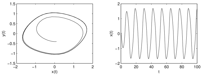
Figure 2: Phase plot and waveform plot for system (9) with $\alpha=0.02$

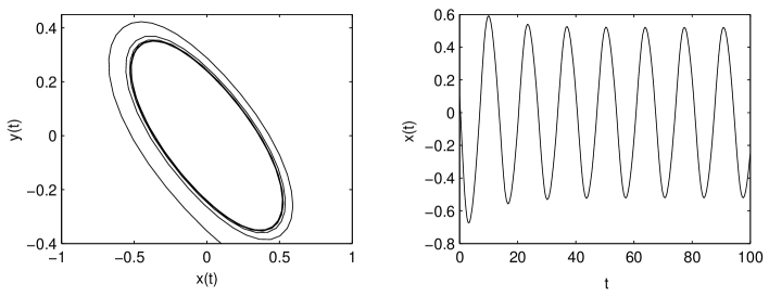
Figure 3: Phase plot and waveform plot for system (9) with $\alpha=0.5$

4 Chaos in an excited tabu learning single neuron model

In this section, the dynamical behaviors of a tabu learning single neuron model, with external sinusoidal input, are studied.

In system (8), let $I$ be

$$I(t)=\epsilon\sin(\omega t)$$

and let the nonlinear activation function be

$$f(x)=pxe^{-(px)^{2}/\sigma^{2}}$$ (13)

where $\epsilon,\,\omega,\,p$, and $\sigma$ are positive constants. Also, in system (8), set the parameters be $C=1,\,R=7,\,a=0.3,\,\epsilon=0.2,\,\omega=2\pi,\,\alpha=0.6,\,\beta=0.9$, and set $p=8,\,\sigma^{2}=0.2$ in (13). It should be noted that several other parameters have also been examined, showing similar dynamical phenomena. Due to the space limitation, those results are not presented here.

The phase plot of $x$ and $y$ and the waveform plot of $x$ are shown in Fig. 4 and Fig. 5, respectively. And in Fig. 6, the power spectrum of the neuron state $x$, calculated using the general FFT, is plotted.

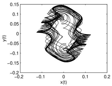
Figure 4: Phase plot

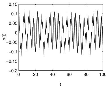
Figure 5: Waveform plot of $x$

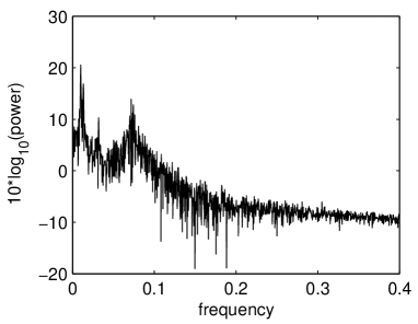
Figure 6: Power spectrum of the time series of $x$

In order to calculate the largest Lyapunov exponent, the method introduced in [Wolf et al., 1985] is used, in which one monitors the long-term evolution of a single pair of nearby orbits. The largest Lyapunov exponent is defined as

$$\lambda=\frac{1}{t_{M}-t_{0}}\sum_{k=1}^{M}\mbox{log}_{2}\frac{L^{\prime}(t_{k})}{L(t_{k-1})}$$

where $M$ is the total number of replacement steps, $L(t_{k-1})$ is the distance between the two initial points at the time instant $t_{k-1}$. After a time step $\delta=t_{k}-t_{k-1}$, the initial length will have evolved to length $L^{\prime}(t_{k})$, as detailed in [Wolf et al., 1985]. In the simulations, the largest Lyapunov exponent $\lambda$ is calculated from a time series of $N=100,000$ points. The largest Lyapunov exponent is obtained as $\lambda=0.7030$.

From Figs. 4-6 and the largest Lyapunov exponent, one can see that there exists chaotic behavior in this nonautonomous tabu learning single neuron model.

5 Chaos in a two-neuron model with a linear proximity function

Now, consider a two-neuron model with a linear proximity function. From (6) and (7), one knows that there are totally four differential equations in this system:

$$\begin{array}[]{rl}C_{1}\dot{u}_{1}=&-\frac{1}{R_{1}}u_{1}+T_{11}V_{1}+T_{12}V_{2}+I_{1}+J_{1}\\ C_{2}\dot{u}_{2}=&-\frac{1}{R_{2}}u_{2}+T_{21}V_{1}+T_{22}V_{2}+I_{2}+J_{2}\\ \dot{J}_{1}=&-\alpha J_{1}-\beta V_{1}\\ \dot{J}_{2}=&-\alpha J_{2}-\beta V_{2}\end{array}$$ (14)

In the following simulations, without loss of generality, let $C_{1}=C_{2}=1$, $R_{1}=R_{2}=10$, $I_{1}=I_{2}=0$, $\alpha=0.1$, $\beta$ be a variable parameter, and let the weight matrix be

$$T=\left[\begin{array}[]{cc}0.1&0.5\\ -1&2\end{array}\right]$$

Moreover, let the activation function be $V_{i}=f(u_{i})=\mbox{tanh}(5u_{i})$. It should be noted that several other parameters have also been examined, showing similar dynamical behaviors. Due to space limitation, those results are not presented here.

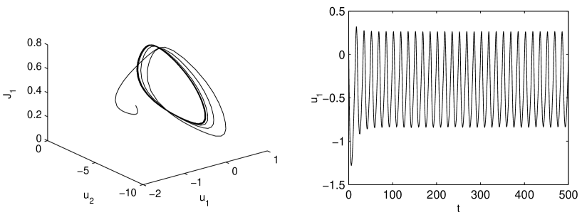
Figure 7: Phase plot and waveform plot of the two-neuron model (14) ($\beta=0.1$)

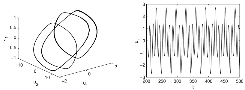
Figure 8: Phase plot and waveform plot of the two-neuron model (14) ($\beta=0.5$)

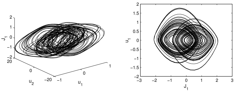
Figure 9: 3-D and 2-D phase plots of the two-neuron model (14) ($\beta=1$)

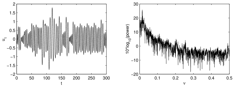
Figure 10: Waveform plot and power spectrum of the two-neuron model (14) ($\beta=1$)

Start from the case of $\beta=0.1$, with which the neural network produces periodic solutions. Fig. 7 shows the 3-D phase plot and the waveform plot of $u_{1}$. Fig. 8 shows the 3-D phase plot and the waveform plot of the network orbit when $\beta=0.5$. In this case, it is also a periodic solution, but it is different from that of the case $\beta=0.1$. When $\beta=1$, the orbit of the neural network is chaotic, and the largest Lyapunov exponent is 0.2419. The 3-D and 2-D plots of the chaotic attractor are shown in Fig. 9. The corresponding waveform and power spectrum are shown in Fig. 10, where the spectrum has been truncated at $\nu$=0.5 HZ.

6 Chaos in a two-neuron model with a quadratic proximity function

If the quadratic proximity function (5) is selected, then the tabu learning neural network that performs gradient descent minimization on $E_{t}$ has the following state equations:

$$\begin{array}[]{lcl}C_{i}\dot{u}_{i}&=&-\frac{1}{R_{i}}u_{i}+\sum_{j}T_{ij}V_{j}+I_{i}-\frac{\partial{F_{t}}(V)}{\partial{V_{i}}}\\ &=&-\frac{1}{R_{i}}u_{i}+\sum_{j}(T_{ij}+S_{ij}(t))V_{j}+I_{i}+J_{i}(t)\end{array}$$ (15)

where

$$\begin{array}[]{rl}S_{ij}(t):=&-\beta\int_{0}^{t}e^{\alpha(s-t)}V_{i}(s)V_{j}(s)\,ds\hskip 14.22636pt(i\neq j)\\ S_{ii}(t):=&0\\ J_{i}(t):=&-\beta(n-1)\int_{0}^{t}e^{\alpha(s-t)}V_{i}(s)\,ds\end{array}$$

in which $n$ is the number of neurons. Therefore, $S_{ij}(t),\,i\neq j$, and $J_{i}(t)$ satisfy the following learning equations:

$$\dot{S}_{ij}=-\alpha S_{ij}-\beta V_{i}V_{j}$$ (16)

$$\dot{J_{i}}=-\alpha J_{i}-\beta(n-1)V_{i}$$ (17)

There are totally six differential equations in this model:

$$\begin{array}[]{rl}C_{1}\dot{u}_{1}=&-\frac{1}{R_{1}}u_{1}+(T_{12}+S_{12}(t))V_{2}+I_{1}+J_{1}(t)\\ C_{2}\dot{u}_{2}=&-\frac{1}{R_{2}}u_{2}+(T_{21}+S_{21}(t))V_{1}+I_{2}+J_{2}(t)\\ \dot{S}_{12}=&-\alpha S_{12}-\beta V_{1}V_{2}\\ \dot{S}_{21}=&-\alpha S_{21}-\beta V_{2}V_{1}\\ \dot{J}_{1}=&-\alpha J_{1}-\beta V_{1}\\ \dot{J}_{2}=&-\alpha J_{2}-\beta V_{2}\end{array}$$ (18)

For this model, only its chaotic behavior is discussed. Let $C_{1}=C_{2}=1$, $R_{1}=R_{2}=10$, $I_{1}=I_{2}=0$, $\alpha=0.1$, $\beta=100$, $V_{i}=\mbox{tanh}(10u_{i})$, and the weight matrix be

$$T=\left[\begin{array}[]{cc}0&30\\ 50&0\end{array}\right]$$

Then, the neural network is chaotic. The 3-D and 2-D phase plots of the chaotic attractor are shown in Fig. 11 and Fig. 12, respectively. The waveform plot and power spectrum of $u_{1}$ are shown in Fig. 13, in which the largest Lyapunov exponent is 0.3160.

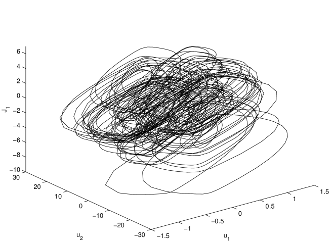
Figure 11: 3-D phase plot of the chaotic attractor of the two-neuron model (18)

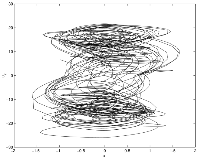
Figure 12: 2-D phase plot of the chaotic attractor of the two-neuron model (18)

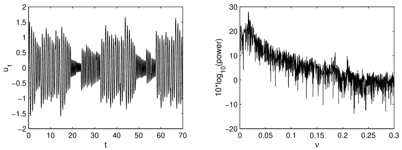
Figure 13: Waveform plot and power spectrum plot of the two-neuron model (18)

7 Conclusions

The nonlinear dynamical behaviors of some tabu learning neuron models have been studied in this paper. By choosing the memory decay rate as a bifurcation parameter, it has been proved that Hopf bifurcation occurs in the single neuron model. The stability of bifurcating periodic solutions and the direction of the Hopf bifurcation are determined based on the normal form theory. From the waveform diagrams, the phase plots, the power spectra, and the largest Lyapunov exponents, one can find chaotic phenomena in the single neuron model with small external sinusoidal input and in the two-neuron models. These tabu learning models, although simple, have rich complex dynamics, and deserve further investigations.

Acknowledgements

This work was supported by the National Natural Science Foundation of China under Grant 60271019, the Youth Science and Technology Foundation of UESTC under Grant YF020207, and the Hong Kong Research Grants Council under the CERG Grant CityU 1115/03E.

References

Babcock, K.L. & Westervelt, R.M. [1987] “Dynamics of simple electronic neural networks”, Physica D 28, 305-316.

Beyer, D.A. & Ogier, R.G. [1991] “Tabu learning: A neural network search method for solving nonconvex optimization problems”, Proc. of the IJCNN (Singapore), 953-961.

Bondarenko, V.E. [1997] “High-dimensional chaotic neural network under external sinusoidal force”, Phys. Lett. A 236, 513-519.

Das, A., Das, P. & Roy, A.B. [2002] “Chaos in a three-dimensional general model of neural network”, Int. J. Bifurcation and Chaos 12, 2271-2281.

Das II, P.K., Schieve, W.C., Zeng, Z.J. [1991] “Chaos in an effective four-neuron neural network”, Phys. Lett. A 161, 60-66.

Gilli, M. [1993] “Strange attractors in delayed cellular neural networks”, IEEE Trans. Circ. Sys. – I, 40, 849-853.

Glover, F. [1989] “Tabu search, part I”, ORSA J. Comput. 1, 190-206.

Glover, F. [1990] “Tabu search, part II”, ORSA J. Comput. 2, 4-32.

Gopalsamy, K., Leung, I. & Liu, P. [1998] “Global Hopf-bifurcation in a neural netlet”, Appl. Math. Comput. 94, 171-192.

Hassard, B. D., Kazarinoff, N.D., & Wan, Y.H. [1981], Theory and Applications of Hopf Bifurcation (Cambridge University Press, Cambridge).

Kepler, T.B., Datt, S., Meyer, R.B., Abbott, L.F. [1990] “Chaos in a neural network circuit”, Physica D 46, 449-457.

Kurten, K.E. & Clark, J.W. [1986] “Chaos in neural systems”, Phys. Lett. A 144, 413-418.

Li, C., Liao, X. & Yu, J. [2003] “Generating chaos by Oja’s rule”, Neurocomputing 55, 731-738.

Li, C., Yu, J., & Liao, X. [2001] “Chaos in a three-neuron hysteresis Hopfield-type neural network”, Phys. Lett. A 285, 368-372.

Liao, X., Wong, K.-W., Leung, C.-S. & Wu, Z. [2001] “Hopf bifurcation and chaos in a single delayed neuron equation with non-monotonic activation function”, Chaos, Solitons and Fractals 12, 1535-1547.

Liao, X., Wong, K.-W. & Wu, Z. [2001] “Bifurcation analysis on a two-neuron system with distributed delays”, Physica D 149, 123-141.

Liao, X. Wu, Z. & Yu, J. [1999] “Stability switches and bifurcation analysis of a neural network with continuous delay”, IEEE Trans. Sys. Man Cybern. – A 29, 692-696.

Lu, H. [2002] “Chaotic attractors in delayed neural networks”, Phys. Lett. A 298, 109-116.

Olien, L. & Belair, J. [1997] “Bifurcations, stability and monotonicity properties of a delayed neural network model”, Physica D 102, 349-363.

Ueta, T. & Chen, G. [2001] “Chaos and bifurcation in coupled networks and their control”, in Controlling Chaos and Bifurcations in Engineering Systems, G. Chen (ed.), (CRC Press, Boca Raton), 581-601.

Wei, J. & Ruan, S. [1999] “Stability and bifurcation in a neural network model with two delays”, Physica D 130, 255-272.

Wolf, A., Swift, J.B., Swinney, H.L., Vastano, J.A. [1985] “Determining Lyapunov exponents from a time series”, Physica D 16, 285-317.

Zou, F. & Nossek, J.A. [1993] “Bifurcation and chaos in cellular neural network”, IEEE Trans. Circ. Sys. – I 40, 166-172.