Meanders and Reconnection-Collision Sequences in the Standard Nontwist Map

Abstract

New global periodic orbit collision/separatrix reconnection scenarios in the standard nontwist map in different regions of parameter space are described in detail, including exact methods for determining reconnection thresholds that are implemented numerically. The results are compared to a break-up diagram of shearless invariant curves. The existence of meanders (invariant tori that are not graphs) is demonstrated numerically for both odd and even period reconnection for certain regions in parameter space, and some of the implications on transport are discussed.

In recent years, area-preserving maps that violate the twist condition locally in phase space have been the object of interest in several studies in physics and mathematics. These nontwist maps show up in a variety of physical models, e.g., in magnetic field line models for reversed magnetic shear tokamaks. An important problem is the determination and understanding of the transition to global chaos (global transport) in these models. Nontwist maps exhibit several different mechanisms: the break-up of invariant tori and separatrix reconnections. The latter may or may not lead to global transport depending on the region of parameter space. In this paper we conduct a detailed study of newly discovered reconnection scenarios in the standard nontwist map, investigating their location in parameter space and their impact on global transport.

I Introduction

In this paper we consider the standard nontwist map (SNM) $M$, as introduced in Ref. del_castillo93 :

$$\begin{split}x_{n+1}&=x_{n}+a\left(1-y^{2}_{n+1}\right)\,,\\ y_{n+1}&=y_{n}-b\sin\left(2\pi x_{n}\right)\,,\end{split}$$ (1)

where $(x,y)\in{\mathbb{T}}\times{\mathbb{R}}$ are phase space coordinates and $a,b\in{\mathbb{R}}$ parameters. This map is area-preserving and violates the twist condition,

$$\frac{\partial x_{i+1}\left(x_{i},y_{i}\right)}{\partial y_{i}}\neq 0\qquad\forall\ (x_{i},y_{i})\,,$$ (2)

along a curve in phase space, called the nonmonotone curve.petrisor01 Some basic concepts used throughout the paper are reviewed in Appendix A.

Nontwist maps are used to describe many physical systems, e.g., magnetic field lines in tokamaks (see, e.g., Refs. balescu98 ; horton98 ; morrison00 ; oda95 ; petrisor03 ; stix76 ; ullmann00 ) and stellaratorsdavidson95 ; hayashi95 (plasma physics); planetary orbits,kyner68 stellar pulsationsmunteanu02 (astronomy); traveling waves,weiss91 ; del_castillo93 coherent structures and self-consistent transportdel_castillo02 (fluid dynamics). Additional references can be found in Refs. apte03 ; del_castillo96 . Apart from their physical importance, nontwist maps are of mathematical interest because important theorems concerning area-preserving maps assume the twist condition, e.g., the KAM theorem and Aubry-Mather theory. Up to now only few mathematical results are known.apte04b ; delshams00 ; franks03 ; moeckel90 ; simo98 Recently, it has been showndullin00 ; vanderweele88 that the twist condition is violated generically in area-preserving maps that have a tripling bifurcation of an elliptic fixed point. For studies of nontwist Hamiltonian flows, we refer the interested reader to Ref. gaidashev04 and references therein.

Remark 1.

Although the SNM is not generic due to its symmetries (see Appendix B), it captures the essential features of nontwist systems with a local, approximately quadratic extremum of the winding number profile.

Nontwist maps of the annulus exhibit interesting bifurcation phenomena: periodic orbit collision and separatrix reconnection. The former, which applies specifically to collisions of periodic orbits of the same period, such as the so-called up and down periodic orbits that occur in the SNM, can be used to calculate torus destruction.del_castillo96 The latter is a global bifurcation when the invariant manifolds of two or more distinct hyperbolic orbits with the same rotation number connect leading to a change in the phase space topology in the nontwist region. We briefly review previous studies of reconnection in nontwist systems.

Howard and Hohshoward84 defined a quadratic nontwist map closely related to Eq. (1) and studied numerically the reconnection of low-order resonances exhibiting homoclinic and vortex-like structures. Defining an average Hamiltonian they predicted the reconnection threshold for period-one and period-two fixed points. Howard and Humpherys extended the study to cubic and quartic nontwist maps.howard95 These reconnection scenarios had been conjectured by Stixstix76 in the context of the evolution of magnetic surfaces in the nonlinear double-tearing instability, and were seen by Gerasimov et al.gerasimov86 in a two-dimensional model of the beam-beam interaction in a storage ring.

The first systematic study of reconnection was done by van der Weele et al.vanderweele88 ; vanderweele90 in the context of area-preserving maps with a quadratic extremum. As far as we know the terminology “nontwist” and “meanders” originates from there.

Del-Castillo-Negrete et al.del_castillo96 devised an approximate criterion for the reconnection threshold of higher-order resonances based on matching the slopes of the unstable manifolds of the reconnecting hyperbolic orbits.

Continuing the work of Carvalho and Almeida,egydio92 Voyatzis et al.voyatzis99 studied reconnection phenomena in nontwist Hamiltonian systems under integrable perturbation with cubic winding number profiles. Applying Melnikov’s method, they showed the transverse intersection of manifolds for arbitrarily small nonintegrable perturbations for one reconnection scenario when the winding number has a local extremum.voyatzis02

The influence of manifold reconnection on diffusion was studied in the region of strong chaos by Corso et al. in a series of papers.corso98 ; corso99 ; corso03 ; prado00

A very different criterion for the reconnection threshold was proposed by Petrisor in Refs. petrisor02 ; petrisor03 : If two hyperbolic orbits have a heteroclinic connection, their actions coincide. As noted in Ref. petrisor02 , for odd-period hyperbolic orbits in the SNM this criterion reduces to the action being zero at the point of reconnection. This criterion was implemented numerically in Ref. wurm04 to estimate some reconnection thresholds for odd-period orbits in the SNM.

Remark 2.

It has been noted that the above result about the equality of actions of reconnecting hyperbolic orbits is only approximately true in the near-integrable limit.llave04

For completion, we mention a few related studies: reconnection phenomena and transition to chaos in the Harper map,saito97 ; shinohara02 degenerate resonances in Hamiltonian systems with $3/2$ degrees of freedom,morozov02 and zero dispersion resonance in the study of underdamped oscillators.soskin97

Key to the analytical and numerical exploration of the standard nontwist map is the map’s invariance under symmetries, reviewed in Appendix B. Of particular significance are the indicator points,shinohara98 fixed points of some of the symmetries of the SNM, whose importance was first recognized by Shinohara and Aizawa. These points were independently re-discovered by Petrisorpetrisor01 in the analysis of the reversing symmetry grouplamb92 of nontwist standard-like area-preserving maps. In Ref. shinohara97 , it was shown that a shearless invariant torus crosses the $x$-axis at two points. This led the authors to devise a criterion to determine the approximate location in the $(a,b)$-parameter space of the break-up of shearless invariant tori for many winding numbers (see Sec. II.5).

Subsequently, based on numerical observations, Shinohara and Aizawashinohara98 used indicator points to propose exact expressions for the collision threshold of even-period orbits and a method to determine numerically the reconnection threshold for odd-period hyperbolic orbits.

The goal of the present paper is to describe reconnection-collision phenomena in detail in all regions of $(a,b)$-parameter space for the standard nontwist map. The details of the two main scenarios (odd-period and even-period) depend crucially on the $(a,b)$-region, and have not been discussed exhaustively up to now. The main tool we use here is the numerical implementation of two criteria for collision thresholds: the analytic one of Ref. shinohara98 and the numerical one of Ref. del_castillo96 . The resulting curves are compared with the $(a,b)$-space break-up diagram (see Sec. II.5), produced by a modified version of Refs. apte03 ; shinohara97 . Early results of this investigation were reported in Ref. wurm04 , and some of them will be elaborated below for completeness.

The paper is organized as follows. We review some basic concepts of nontwist systems and the SNM in Sec. II. Some novel reconnection and collision scenarios for orbits of even and odd periods are described in Sec. III.1 and Sec. III.2, respectively, applying and extending methods from Refs. del_castillo96 ; shinohara98 . The results are discussed in the context of the break-up diagram in Sec. IV. In Sec. V we give our conclusions and indicate some directions of future research. The appendices contain basic definitions and a brief summary of symmetry properties of the SNM.

II Review of nontwist maps

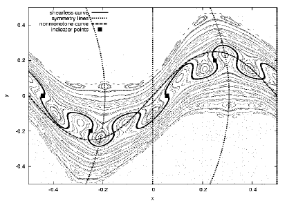
Figure 1: Example of the phase space for standard nontwist map (top) and winding number profile along $y$-axis (bottom) at $a=0.615$, $b=0.4$. The symmetry lines, nonmonotone curve $\cal C$, $\cal G$-invariant curve $\gamma_{S}$, and indicator points are displayed.

In this section, we review some fundamental concepts that are required for further explorations of the SNM. Fig. 1 shows a typical phase space plot along with the plot of winding number $\omega$ versus $y$ (henceforth called winding number profile) for the central section of the $y$-axis.

The phase space of the SNM consists of two twist regions, “above” and “below” the center, i.e., regions in which Eq. (2) is satisfied. Since the twist condition is violated along the nonmonotone curve $\cal C$ given by $y=b\sin(2\pi x)$, only orbits with points falling on $\cal C$, referred to as nonmonotone orbits by Petrisor,petrisor01 and orbits with points on both sides of $\cal C$, called pseudomonotone, are affected by the nontwist property. Note that, for any $b\neq 0$, the curve $\cal C$ is not an invariant torus.

Like the phase space plot, the winding number profile in the outer regions looks the same as that of a twist map, showing, e.g., the familiar plateaus associated with islands around periodic orbits (here orbits with winding numbers 3/5, 7/12, and 4/7). The only distinctly nontwist effect, aside from the existence of the overall maximum (here at 3/5) and of multiple periodic orbits of winding numbers less than the maximum, is the valley below the 3/5 plateau, which gives rise to a variety of phenomena discussed in Sec. III.

II.1 Reversing symmetry group and shearless curve

When the winding number profile has a local extremum at an irrational value of $\omega$, the corresponding invariant torus is called shearless. As discussed by Petrisor,petrisor01 the SNM has at most one homotopically nontrivial shearless invariant torus $\gamma_{S}$ that is also invariant under the reversing symmetry group $\mathcal{G}$ (reviewed in Appendix B). When it exists, $\gamma_{S}$ also contains the indicator points

$$\boldsymbol{z}_{0}^{(0,1)}=\left(\mp\frac{1}{4},\mp\frac{b}{2}\right)\,,\mbox{ and }\boldsymbol{z}_{1}^{(0,1)}=\left(\frac{a}{2}\mp\frac{1}{4},0\right)\,,$$ (3)

and all their iterates. As we will discuss in Sec. III, in some regions of parameter space, there exist several shearless tori, but only one of them is $\mathcal{G}$-invariant.

The significance of a shearless torus is that it acts as a barrier to transport, whereas the nonmonotone curve $\cal C$ does not. Fig. 1 shows the nonmonotone curve and the shearless torus, along with symmetry lines and indicator points.

The standard nontwist map is non-generic because it is time-reversal symmetric as well as invariant under a symmetry, as reviewed in Appendix B. Nevertheless, most of the phase space phenomena described in this paper are also observed in arbitrary nontwist systems, even though the exact definitions of many of the concepts introduced to study them cannot be generalized to these systems.

II.2 Periodic orbit collision and standard separatrix reconnection

As mentioned earlier, one consequence of the violation of the twist condition is that the SNM has more than one orbit (either invariant tori or chains of periodic orbits) of the same winding number. These orbits can collide and annihilate at certain parameter values.

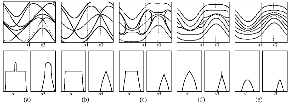
Figure 2: The standard scenario of even-period reconnection/collision sequences (upper row, $y$ vs. $x$) and winding number profiles along the $s_{1}$ and $s_{3}$ symmetry lines (lower row, $\omega$ along $s_{i}$ vs. $y$). (discussion in text)

The collision of periodic orbits involves another purely nontwist phenomenon, namely the reconnection of the invariant manifolds of the corresponding hyperbolic orbits. These reconnection-collision sequences in the SNM are distinctly different for orbits of even and odd periods. Here we will only give a brief account of the simplest version of both sequences, which we will refer to as the standard scenarios.vanderweele90 We show phase space plots and winding number profiles for several steps in these sequences. The description of more intricate reconnection-collision scenarios appears in Secs. III.1 and III.2.

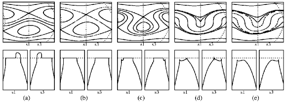
Figure 3: The standard scenario of odd-period reconnection/collision sequences (upper row, $y$ vs. $x$) and winding number profiles along the $s_{1}$ and $s_{3}$ symmetry lines (lower row, $\omega$ along $s_{i}$ vs. $y$). (discussion in text)

Changing the parameter values of the SNM we see the following sequences:

• For orbits with even period, i.e., with the same stability type for both the up and down orbits on a symmetry line (Fig. 2a): collision of the hyperbolic orbits which is also the threshold for reconnection (Fig. 2b); the “dipole topology” in which the hyperbolic orbits have moved off the symmetry lines (Fig. 2c); the collision of elliptic orbits that coincides with the collision of the non-symmetric hyperbolic orbits (Fig. 2d) leading to annihilation of these periodic orbits (Fig. 2e).
  The winding number profile shows a maximum that is greater than, equal to, and less than the winding number of the periodic orbit before, during, and after this process, respectively.

• For orbits with odd period, i.e., with opposite stability type for the up and down orbits on a symmetry line (Fig. 3a): reconnection of hyperbolic manifolds of up and down orbits (Fig. 3b); appearance of non-KAM meandering orbits (elaborated on in Sec. II.4), homoclinic separatrices, and dimerized chains (Fig. 3c); hyperbolic-elliptic collision (Fig. 3d) leading to annihilation of these periodic orbits (Fig. 3e).
  As above, the winding number profile shows a global maximum that is greater than, equal to, and less than the winding number of the periodic orbit before, during, and after this process, respectively. But in addition, there is a local minimum – associated with the appearance of the meandering orbits – which persists even after the collision. (See Sec. II.4.)

II.3 Bifurcation and indicator curves

The parameter values for the threshold of collision of periodic orbits with a fixed winding number are numerically observed to lie on a smooth curve in $(a,b)$-parameter space, called bifurcation curve, which was first defined in Ref. del_castillo96 .

The $m/n$-bifurcation curve $b=\Phi_{m/n,i}(a)$ is the set of $(a,b)$ values for which the $m/n$ up and down periodic orbits on the symmetry line $s_{i}$ (see Appendix B) are at the point of collision. (For clarity, the figures in this paper denote these curves by “bc1,” “bc2” etc. for symmetry lines $s_{1}$, $s_{2}$ etc.) The main property of this curve is that for $(a,b)$ values below $b=\Phi_{m/n,i}(a)$, the $r/s$ periodic orbits, with $r/s<m/n$, exist. Thus, $m/n$ is the maximum winding number for parameter values along the $m/n$-bifurcation curve.

For $n$ odd, bifurcation curves along $s_{1}$ through $s_{4}$ coincide in the SNM because of the map’s high degree of symmetry. For $n$ even, bifurcation curves along $s_{1}$ and $s_{2}$ are separate from the ones along $s_{3}$ and $s_{4}$ for any $b\neq 0$.

	Elliptic collision	Hyperbolic reconnection
$\omega=\frac{1}{2}$	$a=\frac{1}{2}$	$b^{2}=4\left(1-\frac{1}{2a}\right)$
$\omega=\frac{1}{4}$	$b^{2}=\frac{2}{\cos^{2}(a\pi)}\left(1-\frac{1}{4a}\right)$	$b^{2}=4\left(1-\frac{1}{4a}\right)$
$\omega=\frac{1}{6}$	$b^{2}=\frac{3}{2\cos^{2}(a\pi)}\left(1-\frac{1}{6a}\right)$	$b^{2}=\frac{\left(1-\frac{1}{6a}\right)}{\left[2+\left(1+2\cos\left(2\pi a\left(1-\frac{b^{2}}{4}\right)\right)\right)\right]}$

Table 1: Some exact expressions for indicator curves for even-period orbits.

Shinohara and Aizawashinohara98 used the numerical observation that at the point of hyperbolic collision (Fig. 2b) for even-period orbits (but not for the odd-period case), two of the indicator points belong to the hyperbolic periodic orbit. This implies that (for period $2n$)

$$M^{2n}\boldsymbol{z}_{j}^{(0,1)}=\boldsymbol{z}_{j}^{(0,1)}$$ (4)

for either $j=0$ or $j=1$, where $\boldsymbol{z}_{j}^{(0,1)}$ are given in Eq. (3). The symmetries of the map further imply that the indicator points map onto each other after $n$ iterations, i.e.,

$$M^{n}\boldsymbol{z}_{j}^{(0,1)}=\boldsymbol{z}_{j}^{(1,0)}\,.$$ (5)

By solving these equations for the two unknowns $(a,b)$, we can obtain exact expressions for the bifurcation thresholds. Some of the resulting curves for low-period orbits are given in Table 1. They are related to the ones given in Ref. shinohara98 by a simple transformation.

We will later see that when more than two chains of periodic orbits exist, the collision threshold for some of them, but not for the others, is given by the above criterion. Hence we will find it useful to introduce the notion of indicator curves $b=\Psi_{m/n}(a)$ defined by (4) (or (5)) . When only two chains of $m/n$-orbits exist, either $\Phi_{m/n,1}$ or $\Phi_{m/n,3}$ coincides with $\Psi_{m/n}$. Hence we label indicator curves by symmetry lines, e.g., $\Psi_{m/n,1}$. (We will denote these curves by “ic1” and “ic3” in the figures for clarity.)

Remark 3.

Shinohara and Aizawa also proposed a numerical criterion to find the odd-period reconnection threshold. They discovered numerically that at the threshold successive iterates of indicator points approach the same hyperbolic periodic point of the reconnecting chains. For details see Ref. shinohara98 .

II.4 Meandering orbits

Another characteristic of nontwist maps is the occurrence of meandering orbits, which are readily observed in the standard reconnection-collision scenario for odd-period orbits, but not in the one for even-period orbits. (For non-standard even-period reconnection-collision scenarios in which meanders occur, see Sec. III.1.) As seen in Fig. 3c (and also in Fig. 1), in the region surrounding $\gamma_{S}$, confined by two dimerized chains, new periodic orbits and non-KAM tori appear, i.e., orbits and tori that did not exist at zero perturbation ($b=0$). These tori are not graphs over the $x$-axis and have been called meanders or meandering curves.simo98 ; vanderweele88 Such invariant tori can occur only in nontwist maps because any invariant torus for a twist map must be a graph over $x$.

It is observed numerically that in the meandering region the winding numbers of the meandering orbits are less than the winding number of the reconnecting periodic orbits. Conversely, however, a “valley” in the winding number profile does not imply the existence of meanders as seen, e.g., in Fig. 3e. The existence of the local minimum and the valley leads to four or more chains of periodic orbits for certain winding numbers. We will discuss in Sec. III.1 and Sec. III.2 the reconnection and bifurcation phenomena in this scenario, which we call the non-standard scenario.

II.5 Break-up diagram

Since the shearless curve $\gamma_{S}$, whenever it exists, poses a barrier to transport between the two twist regions, studying its break-up is of considerable practical interest. Highly detailed studies of break-up of shearless curves were conducted for a few winding numbers using Greene’s residue criterion.apte03 ; apte04 ; del_castillo96 Though the method is very precise, it is not suitable for an exploration of all parameter space. Shinohara and Aizawashinohara97 obtained a rough estimate for the break-up threshold of many shearless curves by investigating for a range of parameter values whether iterates of one of the indicator points remain bounded.

Here, we implement the following slightly different strategy, using the fact that if the winding number of the orbit of any point exists, then the orbit is not chaotic – it is either periodic or quasiperiodic. We calculate the sequence $\omega_{i}=x_{i}/i$ for the iterates $(x_{i},y_{i})=M^{i}(\boldsymbol{z})$ of one of the indicator points $\boldsymbol{z}_{j}^{(0,1)}$. The winding number is assumed to exist if we can find some $N$ such that $|\omega_{i}-\omega_{i+1}|<\epsilon,\ \sup_{n<N}\ \omega_{n}>\omega_{i}$, and $\inf_{n<N}\ \omega_{n}<\omega_{i}$ for $N<i<N+M$. We use $\boldsymbol{z}=(a/2+1/4,0),\ \epsilon=10^{-7},\ M=10^{5}$, and the maximum $N$ used is $2.9\times 10^{6}$. If the winding number sequence displays larger fluctuations, we assume the orbit to be chaotic, i.e., the torus to be destroyed. This criterion is also only approximate, since the value of the winding number might converge for the number of iterations used, but further iterations would reveal fluctuations, or vice versa.

The method of Ref. shinohara97 and ours deliver similar results. However, it seems that the computation of the winding number provides better means of monitoring and controlling its accuracy (aside from giving us the winding number of the shearless curve as a useful side-product).

The boundary of the resulting break-up diagram displays a fractal-like structure (see, e.g., Fig. 11). The analysis of Refs. apte03 ; del_castillo96 ; shinohara97 indicates that the highest peaks correspond to the break-up of shearless invariant tori with noble winding numbers (see Refs. apte03 ; apte04 for discussion). We will comment in Sec. IV on the relation between the break-up diagram, reconnection, and the indicator and bifurcation curves.

III Non-standard reconnection and collision scenarios

As noted in Sec. II.4, the winding number profile can have a valley and a local minimum (denoted by $\omega_{\text{min}}$) between two local maxima (denoted by $\omega_{\text{max}}\leq\omega^{\prime}_{\text{max}}$). (In many cases it is observed that $\omega_{\text{max}}=\omega^{\prime}_{\text{max}}$, so we will not distinguish between the two maxima.) Thus there are four orbits for each winding number in the range $\omega_{\text{min}}<\omega<\omega_{\text{max}}$. The maxima and the minimum are seen to decrease when the perturbation, $b$, is increased. This gives rise to the following scenarios for reconnection and collision of $m/n$-periodic orbits:

• For $\omega_{\text{min}}>m/n$, there are two chains of $m/n$-periodic orbits.

• When $\omega_{\text{min}}$ reaches the rational value $m/n$, periodic orbits of winding number $m/n$ are born and subsequently reconnect, in addition to already existing orbits. We call the new orbits inner orbits while the already existing ones will be called outer orbits.

• When $\omega_{\text{max}}$ reaches $m/n$, the inner orbits reconnect and collide with the outer orbits.

• For $\omega_{\text{max}}<m/n$, no $m/n$-periodic orbits exist.

The reconnections and collisions that occur in the above scenario are locally the same as those seen in Sec. II.2. But because of the presence of four chains of periodic orbits, the global topology is considerably more complicated as will be seen below.

Remark 4.

A valley in the winding number profile shows up after reconnection, together with meandering orbits, and also persists after the collision of the reconnecting orbits (Fig. 3e). The scenario described in the above paragraph typically occurs for parameter values slightly above (in $b$ vs. $a$ parameter space plots) the bifurcation curves of odd-period orbits.

Remark 5.

When a valley in the winding number profile exists, the winding number of the shearless curve is the local minimum $\omega_{\text{min}}$, if $\omega_{\text{min}}$ is irrational.

Remark 6.

When $\omega_{\text{min}}=m/n$, the reconnection process of the inner (meandering) orbits involves orbits, called second-order meanders,simo98 that meander around these inner orbits. The winding number profile shows a “hill” at the bottom of the valley. Such a process might give rise to arbitrarily higher order meanders.petrisor01 ; simo98 ; wurm04

III.1 Non-standard scenarios for even-period orbits

A first hint that for the non-generic SNM the even-period reconnection scenario can be more complicated is found in Ref. shinohara98 . In some region of $(a,b)$-parameter space, phase space portraits show the appearance of meanders and additional periodic orbits.

Figure 4: Indicator curves (ic1 and ic3) and bifurcation curves (bc1 and bc3) for 7/8 periodic orbits.

For most regions of $(a,b)$-space the indicator and bifurcation curves are seen to coincide. But in regions of parameter space where the winding number profile has a valley, bifurcation curves and indicator curves separate (and can even cross each other) leading to various reconnection scenarios and the appearance of meanders.

This is seen most clearly near $a=1$, which is the bifurcation curve for the $1/1$-periodic orbits, but, as mentioned above, occurs above every odd-period bifurcation curve. We discuss in detail the example of $7/8$-periodic orbits, whose indicator and bifurcation curves are shown in Fig. 4 for the parameter space region of interest.

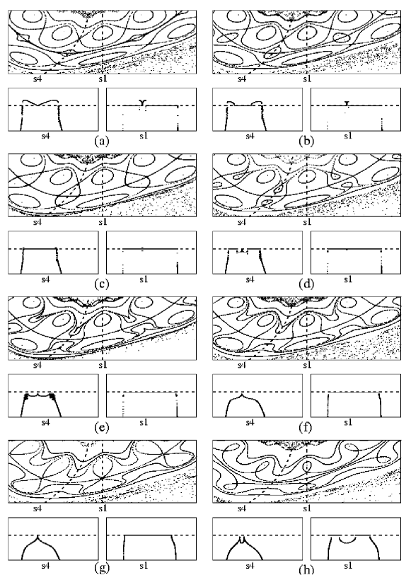
Figure 5: 7/8-orbit reconnection at $a=0.923$ (discussion in text). The upper plot shows a $y$ vs. $x$ phase space plot ($x\in[-0.25,0.25],y\in[-0.5,0]$) and the lower one the corresponding winding number profiles along the two indicated symmetry lines ($\omega$ along $s_{i}$ vs. $y$, $\omega\in[7/8-0.0007,7/8+0.0005]$). The plots correspond to the $b$-values: a) 0.22325262 $(\approx\Psi_{3})$, b) 0.22335, c) 0.22346060, d) 0.22355, e) 0.22364169 $(\Phi_{3})$, f) 0.22385, g) 0.22416343 $(\Psi_{1})$, h) 0.22465.

For approximately $a<0.92$, the curves coincide, resulting in the standard scenario (Sec. II.2). The lower curve, corresponding to bc3 and ic3, is the threshold for collision (i.e., reconnection) of hyperbolic orbits, while the upper curve, corresponding to bc1 and ic1, is for the simultaneous collision (annihilation) of elliptic and non-symmetric hyperbolic orbits. For $a>0.92$ the curves separate, and around $a=0.925$ the bifurcation curve bc3, crosses the indicator curve ic1.

Recall that $b=\Phi_{7/8,i}(a)$ is the bifurcation curve for orbits on the symmetry line $s_{i}$, and $b=\Psi_{7/8,i}(a)$ is the indicator curve. In the following we drop the subscript $7/8$ and the dependence on $a$. Also, the symmetry of the SNM implies that $\Phi_{1}=\Phi_{2}$ and $\Phi_{4}=\Phi_{3}$.

The separation gives rise to the following two sequences:

For $0.92<a<0.925$, the above curves are in the following order: $\Psi_{3}<\Phi_{3}<\Psi_{1}<\Phi_{1}$.

1. Whereas for small perturbations ($b<\Psi_{3}$), only the up and down (outer) $7/8$-chains exist ($\omega_{\text{min}}>7/8$), $\omega_{\text{min}}$ reaches $7/8$ and inner orbits are born at $b=\Psi_{3}$ (Fig. 5a). Initially, this inner chain has the dipole topology, with elliptic orbits on $s_{3}$ and $s_{4}$, and hyperbolic orbits not on any symmetry line. (Fig. 5b).

2. Somewhere in the range $\Psi_{3}<b<\Phi_{3}$, a reconnection between these off-symmetry line hyperbolic orbits with the outer hyperbolic orbits on $s_{3}$ and $s_{4}$ occurs (Fig. 5c). At the point of reconnection, $\omega_{\text{max}}$ is $7/8$ and continues to be so through step 5. After this reconnection, meanders are born, the inner and outer chains display a nested topology, and $\omega_{\text{min}}<7/8$ (Fig. 5d).

3. The inner elliptic orbits collide with the outer hyperbolic orbits on the $s_{3}$ and $s_{4}$ symmetry line at $b=\Phi_{3}$ (Fig. 5e), leaving only the off-symmetry line inner hyperbolic orbits and the outer elliptic orbits on the symmetry lines $s_{1}$ and $s_{2}$ (Fig. 5f).

4. At $b=\Psi_{1}$, the inner hyperbolic orbits collide (Fig. 5g) and move onto the symmetry lines $s_{1}$ and $s_{2}$ (Fig. 5h).

5. At $b=\Phi_{1}$, there is an hyperbolic-elliptic collision on $s_{1}$ and $s_{2}$, after which $7/8$-periodic orbits cease to exist and $\omega_{\text{max}}<7/8$.

For $a>0.925$, the order of the curves is changed to $\Psi_{3}<\Psi_{1}<\Phi_{3}<\Phi_{1}$. Most steps of the above sequence remain the same (with $\Psi_{1}$ replacing $\Phi_{3}$ in the second step), except for the following:

1. At $b=\Psi_{1}$, the inner hyperbolic orbits collide and move onto the symmetry lines $s_{1}$ and $s_{2}$, while the hyperbolic elliptic orbits on $s_{3}$ and $s_{4}$ merely continue to approach each other.

2. The inner elliptic orbits collide with the outer hyperbolic orbits on $s_{3}$ and $s_{4}$ at $b=\Phi_{3}$, leaving only the hyperbolic and elliptic orbits on $s_{1}$ and $s_{2}$.

The difference between the two scenarios is the order in which the collision along $s_{3}$ and $s_{4}$ and the move of the hyperbolic points onto $s_{1}$ and $s_{2}$ occur. Both occur simultaneously for the $(a,b)$-value at which $\Phi_{3}$ and $\Psi_{1}$ intersect.

As in the standard scenario of odd-period orbits, meanders appear in this case when the maximum of the winding number profile is rational. But now there are two meandering regions, and none of the meanders are are $\mathcal{G}$-invariant (Fig. 5e, along $s_{4}$).

Note that the indicator curves, which are obtained using the symmetries of the map, track collisions occurring along the $\mathcal{G}$-invariant curve while the bifurcation curves track the collisions occurring at maxima in the winding number profile, which may or may not be shearless.

This motivates an extension of the definition of bifurcation curves. Recall that in the original definition the bifurcation curve determines the global boundary in parameter space between existence and non-existence of periodic orbits of the corresponding winding number. These curves correspond to maxima in the winding number plot, and will be denoted by $\Phi^{\text{out}}_{m/n,i}$ from now on.

In the region of parameter space where four (or more) orbits of a particular winding number exist, a new kind of bifurcation curve can be defined that corresponds to parameter values at which the inner orbits are born, denoted by $\Phi^{\text{in}}$. In this case, the winding number profile has a local minimum (or local maximum for higher order curves). For even-period orbits, as expected and verified numerically, $\Psi_{i}=\Phi_{i}^{\text{in}}$ .

Figure 6: Boundary of break-up diagram (dots), indicator curves (ic) and bifurcation curves (bc) for two different winding numbers. Points marked ($\bullet$) correspond to points where $\Phi^{\text{out}}_{1}$ and $\Phi^{\text{in}}_{1}$ of close-by periodic orbits separate.

Figure 7: Boundary of break-up diagram (dots) and bc1 for $1/3$-orbits (top) and $2/3$-orbits (bottom). Points marked ($\bullet$) correspond to points where $\Phi^{\text{out}}_{1}$ and $\Phi^{\text{in}}_{1}$ of close-by periodic orbits separate.

To estimate the region of parameter space in which there are more than two chains of periodic orbits, we plot the points of separation of indicator and bifurcation curves for several different (odd and even) winding numbers. The results are shown in Fig. 6. Within numerical uncertainty, close to the $1/1$-bifurcation curve the points seem to lie on a curve. Similar “curves” have been numerically observed for a few other winding numbers, e.g., Fig. 7, where we mark the points at which the indicator curves split from the bifurcation curves (along $s_{1}$) for several inner orbits, in the region of parameter space close to the $1/3$-orbit (left) and $2/3$-orbit (right) bifurcation curve (also shown).

Remark 7.

In Ref. petrisor03 Petrisor et al.  conjectured that in generic nontwist maps the dipole formation scenario for even-period orbits does not occur. Instead, their numerical studies showed that one of the elliptic chains bifurcates, creating and subsequently destroying a saddle-center pair, which has the effect of aligning the elliptic points of one chain with the hyperbolic points of the other one. Reconnection occurs then according to the standard scenario for odd-period reconnection.

III.2 Non-standard reconnection for odd-period orbits

Figure 8: Magnification of split region in parameter space for 8/9-bifurcation curves. The curves appear in the order $\Phi^{\text{in}}<\Phi^{\text{out,up}}_{1}<\Phi^{\text{out,down}}_{1}$. (discussion in text)

Since there is no analog of the criterion Eq. (5) for the odd-period orbits, we cannot define indicator curves for these orbits. But we note that the indicator curves for even-period orbits are the bifurcation curves for the inner orbits, $\Psi_{i}=\Phi_{i}^{\text{in}}$. Thus, we have implemented a version of the numerical method for finding bifurcation curvesapte03 ; del_castillo96 for both the inner and outer orbits in the parameter space region where more than two chains exist. Fig. 6 shows the bifurcation curves for the outer orbits, $b=\Phi_{8/9,i}^{\text{out}}(a)$, and inner orbits, $b=\Phi_{8/9,i}^{\text{in}}(a)$, of winding number $8/9$. (Recall that in the odd-period standard scenario the bifurcation curves, $\Phi^{\text{out}}_{i}$, are the same for all four symmetry lines.) For the remainder of this section, we will drop the dependence on $a$ and the subscript $8/9$ for brevity.

A magnification of $(a,b)$-space around the separation point (Fig. 8) reveals the birth of a new hyperbolic-elliptic pair of periodic orbits along each of the symmetry lines at $b=\Phi^{\text{in}}$ for $a>0.9295$ (lowest curve in Fig. 8). This pair of orbits moves apart and eventually collides/annihilates with the outer, up and down, orbits on the symmetry lines. These collisions do not occur simultaneously in parameter space (in contrast to the even case), which explains the existence of two outer bifurcation curves along each symmetry line, one for the outer up orbit and one for the outer down orbit, denoted by $\Phi^{\text{out,up}}_{i}$ and $\Phi^{\text{out,down}}_{i}$, respectively. Because of the symmetry of the SNM, $\Phi^{\text{out,up}}_{\text{1 and 2}}=\Phi^{\text{out,down}}_{\text{3 and 4}}$ and $\Phi^{\text{out,down}}_{\text{1 and 2}}=\Phi^{\text{out,up}}_{\text{3 and 4}}$.

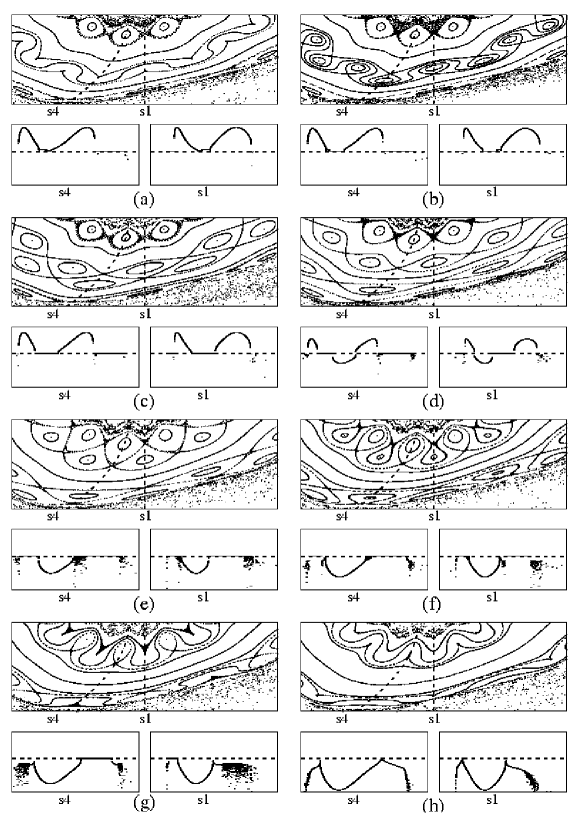
Figure 9: 8/9-orbit reconnection at $a=0.94$ (discussion in text). The upper plot shows a $y$ vs. $x$ phase space plot ($x\in[-0.25,0.25],y\in[-0.5,0]$) and the lower one the corresponding winding number profiles along the two indicated symmetry lines ($\omega$ along $s_{i}$ vs. $y$, $\omega\in[8/9-0.0020,8/9+0.0016]$). The plots correspond to the $b$-values: a) 0.2015781 $(\approx\Phi^{\text{in}})$, b) 0.2018, c) 0.202155, d) 0.2036, e) 0.20515, f) 0.2059, g) 0.2067917 $(\approx\Phi_{1}^{\text{out,up}})$, h) 0.2081084 $(\approx\Phi_{1}^{\text{out,down}})$.

Figure 10: Magnification of the winding number profiles along $s_{1}$ of Figs. 9a (top) and 9b (bottom)..

To illustrate this non-standard reconnection-collision sequence, we discuss in some detail the case of $8/9$-periodic orbits along $s_{1}$ at $a=0.94$ (Fig. 9):

1. Whereas for small perturbations ($b<\Phi^{\text{in}}$), only the up and down (outer) orbits exist and $\omega_{\text{min}}>8/9$, inner chains of orbits are born (Fig. 9a) at $b=\Phi^{\text{in}}$, and subsequently form a nested topology with meandering orbits (Fig. 9b). As seen in the corresponding winding number profile along $s_{1}$, the bottom of the valley exhibits a hill whose edges have the value $\omega_{\text{min}}=8/9$. The left edge, corresponding to the new periodic orbit pair, broadens as its hyperbolic and elliptic orbits start to move apart (Fig. 10), whereas the right one, corresponding to the heteroclinic connection between new pairs on other symmetry lines, continues to touch $\omega_{\text{min}}=8/9$ at only one point. The winding number of the shearless curve, corresponding to the local maximum (top of hill), and those of the meandering orbits are greater than $8/9$.

2. Somewhere in the range $\Phi^{\text{in}}<b<\Phi^{\text{out,up}}_{1}$, the nested orbits reconnect (Fig. 9c), resulting in four regular Poincaré-Birkhoff chains (Fig. 9d), two on each side of the central shearless curve.

3. At a higher $b$-value in the same range, the two up chains and two down chains reconnect (Fig. 9e), resulting in two regions of nested orbits with meandering tori (Fig. 9f). Again, the winding numbers of the meanders is less than that of the reconnecting orbits ($8/9$). Each of these regions contains a shearless, but not $\mathcal{G}$-invariant, meander.

4. At $b=\Phi^{\text{out,up}}_{1}$, the outer up orbits undergo a hyperbolic-elliptic collision (Fig. 9g).

5. At $b=\Phi^{\text{out,down}}_{1}$, the outer down orbits undergo a hyperbolic-elliptic collision (Fig. 9h), after which no further $8/9$-periodic orbits exist.

IV Discussion

To understand the effect of the different reconnection-collision scenarios on the global transport properties of the map, we compare the computed bifurcation and indicator curves with the break-up diagram, obtained using the procedure of Sec. II.5. The results are presented in Fig. 11. We see that these curves serve as a scaffolding for the diagram, an observation also made in Refs. shinohara98 ; wurm04 .

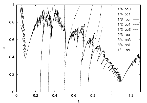
Figure 11: Parameter space showing the points for which shearless invariant tori exist. Also shown are some bifurcation and indicator curves and the critical points (marked by $\circ$) found using Greene’s residue criterion.

Figure 12: Section of parameter space around the $5/6$-orbit indicator and bifurcation curves.

We will illustrate this interplay between the different reconnection scenarios and transition to global chaos by looking at the magnification of the break-up diagram around the indicator and bifurcation curves of the $5/6$-orbits (Fig. 12).

• For approximately $a<0.883$, indicator and bifurcation curves along the different symmetry lines coincide, and lie within the non-chaotic region of the break-up diagram. Fixing $a$ and increasing the perturbation $b$ through the reconnection process does not lead to global chaos. This is because of the presence of invariant tori “above” and “below” the reconnecting chains of orbits. (For the remaining discussion, we will refer to these as ”twist” tori.)

• For approximately $0.883<a<0.893$, the lower pair of curves follows the boundary of the break-up diagram. Increasing the perturbation through the boundary corresponds to a reconnection that results in global chaos. The reason for this can be understood as follows: For parameter values slightly below the lower pair of curves, no twist invariant tori exist above or below the shearless region. Only the tori in the region between the two chains of $5/6$-orbits inhibit transport. When the perturbation $b$ reaches the lower pair of curves, the hyperbolic $5/6$-orbits collide and the tori between the two chains are destroyed. Since the colliding orbits are hyperbolic, their separatrices form a heteroclinic tangle that connects the up and down chaotic regions resulting in global chaos, consistent with the observation that the lower pair of curves form a boundary of the break-up diagram.

• For approximately $0.893<a<0.91$, we see the first of the two non-standard scenarios (Fig. 5) discussed in Sec. III.1. Here again, no twist tori exist for parameter values close to the lowest curve $\Psi_{3}$. The inner orbits, which are born at $b=\Psi_{3}$, move apart and reconnect with the outer hyperbolic orbits for some $\Psi_{3}<b<\Phi_{3}$. At this point, global chaos ensues because the up and down chaotic regions are joined through the reconnecting invariant manifolds. Thus the lower boundary of the break-up diagram lies between $\Psi_{3}$ and $\Phi_{3}$.
  Also, for $b>\Psi_{1}$, the off-symmetry line hyperbolic orbits move onto the $s_{1}$ symmetry line and their invariant manifolds are no longer connected (“de-connection”). Meandering orbits are created as these hyperbolic orbits move apart along $s_{1}$. These meandering orbits (Fig. 5h) inhibit global chaos. Thus, $b=\Psi_{1}$ (seen as the threshold for “de-connection”) forms the upper boundary of the break-up diagram.

• It was noted in Ref. wurm04 that if the up and down twist regions of the map exhibit chaos when the odd-period orbits reconnect, the reconnection leads to global chaos for the above-mentioned reason (i.e., because of the heteroclinic tangle of the invariant manifolds).

Thus we see that, in general, reconnection (and the break-up of twist tori) has a significant effect on the transition to global chaos. Many, if not all, of the “smooth” boundaries of the break-up diagram can be conjectured to be the result of reconnections of invariant manifolds. Indeed, the reconnections of orbits with higher periods can give rise to finer structures in the break-up diagram. Thus, the “fractal” nature of this diagram might be related to the reconnections in phase space happening at smaller and smaller scales. A reliable criterion for determining the reconnection threshold and its numerical implementation will be extremely useful for testing these ideas.

V Conclusion

In this paper we presented a unified view of various bifurcations and reconnections that occur in the standard nontwist map, but are not observed in twist maps. The bifurcations are locally of three types: collision and annihilation of hyperbolic-elliptic orbit pairs, collision of two symmetric hyperbolic orbits resulting in two non-symmetric hyperbolic orbits, and the simultaneous (in parameter and phase space) collision and annihilation of two hyperbolic and two elliptic orbits. The latter is seen only in the SNM (and closely related maps) because of its high degree of symmetry. The two former bifurcations are observed in all nontwist maps.

We have demonstrated that the non-generic standard nontwist map has more types of periodic orbit reconnection scenarios than previously known, resulting from the presence of four (or more) chains of periodic orbits of the same winding number. Meandering tori, associated with the odd-period reconnection in the SNM, have been shown to exist for certain regions of parameter space for non-standard even-period reconnection. Petrisor and co-workerspetrisor03 have started to compile a list of possible reconnection scenarios for nontwist maps. Our investigation contributes new global scenarios for the case of nontwist maps with a reversing symmetry group, including a spatial symmetry.

We also conjecture (and present heuristic observations) that the reconnection of hyperbolic separatrices leads to global chaos if no “twist” tori exist in the region “outside” the reconnecting chains of orbits. Determination of the break-up threshold of the last twist tori and a precise criterion for calculating reconnection thresholds will shed more light on the accuracy and usefulness of these observations.

VI Acknowledgments

This research was in part supported by U.S. Department of Energy Contract No. DE-FG01-96ER-54346 and by an appointment of A. Wurm to the U.S. Department of Energy Fusion Energy Postdoctoral Research Program administered by the Oak Ridge Institute for Science and Education.

Appendix A Basic definitions

For reference, we list a few basic definitions used throughout the main text. An orbit of an area-preserving map $M$ is a sequence of points $\left\{\left(x_{i},y_{i}\right)\right\}_{i=-\infty}^{\infty}$ such that $M\left(x_{i},y_{i}\right)=\left(x_{i+1},y_{i+1}\right)$. The winding number $\omega$ of an orbit is defined as the limit $\omega=\lim_{i\to\infty}(x_{i}/i)$, when it exists. Here the $x$-coordinate is “lifted” from ${\mathbb{T}}$ to ${\mathbb{R}}$. A periodic orbit of period $n$ is an orbit $M^{n}\left(x_{i},y_{i}\right)=\left(x_{i}+m,y_{i}\right)$, $\forall\>i$, where $m$ is an integer. Periodic orbits have rational winding numbers $\omega=m/n$. An invariant torus is a one-dimensional set $C$ that is invariant under the map $C=M(C)$. Of particular importance are the invariant tori that are homeomorphic to a circle and wind around the $x$-domain because, in two-dimensional maps, they act as transport barriers. Orbits belonging to such a torus generically have irrational winding number.

Appendix B Symmetry properties of the SNM

In this appendix, we review the symmetry properties of the SNM. A detailed discussion of these types of symmetries in general can be found in Ref. lamb98 and, in the context of nontwist systems, in Ref. petrisor01 .

The standard nontwist map $M$ is time-reversal symmetric with respect to two involutions $I_{0}$ and $I_{1}$, i.e., $M^{-1}=I_{i}^{-1}\ M\ I_{i}$, $I_{i}^{2}={\rm Id}$, for $i=0,1$. It then follows that the SNM can be decomposed as $M=I_{1}\circ I_{0}$. In addition, $M$ is also symmetric under an involution $S$ which commutes with both $I_{i}$, i.e., $M=S^{-1}\ M\ S$, $S^{2}={\rm Id}$, and $S\ I_{i}=I_{i}\ S$. The involutions have the following form: $I_{0}(x,y)=(-x,y-b\sin(2\pi x))$, $I_{1}(x,y)=(-x+a(1-y^{2}),y)$, and $S(x,y)=(x+1/2,-y)$.

Since the $I_{i}$ are orientation reversing, their fixed point sets, $\Gamma_{i}=\left\{(x,y)|I_{i}(x,y)=(x,y)\right\}$, are one-dimensional sets, called the symmetry lines of the map. For the SNM, $\Gamma_{0}$ consists of $s_{1}=\left\{(x,y)|x=0\right\}$, $s_{2}=\left\{(x,y)|x=1/2\right\}$, while $\Gamma_{1}$ consists of $s_{3}=\left\{(x,y)|x=a\left(1-y^{2}\right)/2\right\}$, $s_{4}=\left\{(x,y)|x=a\left(1-y^{2}\right)/2+1/2\right\}$.

It is easy to check that $S$ does not have any fixed points. Symmetry lines are useful because the numerical search for symmetric periodic orbits, i.e., orbits with a point belonging to one of the symmetry lines, is a one-dimensional root finding problem and hence considerably easier than the search for non-symmetric orbits.greene68 ; devogel58 For the SNM, there are generally two orbits along any symmetry line of any winding number, called the up and down orbits.

The SNM is time-reversal symmetric with respect to maps $SI_{i}$ as well. The fixed point sets of these orientation preserving maps consist of points in phase space, called indicator points. For the SNM, fixed points of $SI_{0}$ and $SI_{1}$ are, respectively, $\boldsymbol{z}_{0}^{(0,1)}=\left(\mp\frac{1}{4},\mp\frac{b}{2}\right)$, and $\boldsymbol{z}_{1}^{(0,1)}=\left(\frac{a}{2}\mp\frac{1}{4},0\right)$.

The involutions $I_{0}$, $I_{1}$, $S$, and their products form a group $\cal G$ called the reversing symmetry group. There is at most one homotopically nontrivial invariant torus that is invariant under the action of $\cal G$petrisor01 . This torus is called the central or $\mathcal{G}$-invariant shearless torus $\gamma_{S}$. The indicator points belong to $\gamma_{S}$ when it exists.shinohara97 ; shinohara98 ; petrisor01

References

- (1) D. Del-Castillo-Negrete and P. J. Morrison, Phys. Fluids A 5, 948 (1993).
- (2) E. Petrisor, Int. J. of Bifur. and Chaos 11, 497 (2001).
- (3) R. Balescu, Phys. Rev. E 58, 3781 (1998).
- (4) W. Horton, H. B. Park, J. M. Kwon, D. Strozzi, P. J. Morrison, and D. I. Choi, Phys. Plasmas 5, 3910 (1998).
- (5) P.J. Morrison, Phys. Plasmas 7, 2279 (2000).
- (6) G. A. Oda and I. L. Caldas, Chaos, Solit. and Fract. 5, 15 (1995).
- (7) E. Petrisor, J. H. Misguich, D. Constantinescu, Chaos, Solit. and Fract. 18, 1085 (2003).
- (8) T. H. Stix, Phys. Rev. Lett. 36, 10 (1976).
- (9) K. Ullmann and I. L. Caldas, Chaos, Solit. and Fract. 11, 2129 (2000).
- (10) M.G. Davidson, R.L. Dewar, H.J. Gardner and J. Howard, Aust. J. Phys.48, 871 (1995).
- (11) T. Hayashi, T. Sato, H. J. Gardner, and J. D. Meiss, Phys. Plasmas 2, 752 (1995).
- (12) W.T. Kyner, Mem. Am. Math. Soc. 81, 1 (1968).
- (13) A. Munteanu, E. García-Berro, J. José, E. Petrisor, Chaos 12, 332 (2002).
- (14) J. B. Weiss, Phys. Fluids A 3, 1379 (1991).
- (15) D. Del-Castillo-Negrete and Marie-Christine Firpo, Chaos 12, 496 (2002).
- (16) A. Apte, A. Wurm, and P. J. Morrison, Chaos 13, 421 (2003).
- (17) D. Del-Castillo-Negrete, J. M. Greene, and P. J. Morrison, Physica D 91, 1 (1996).
- (18) A. Apte, R. de la Llave and N. Petrov, submitted to Nonlinearity (2004), (draft available at http://www.ma.utexas.edu/mp_arc-bin/mpa?yn=04-320).
- (19) A. Delshams and R. de la Llave, SIAM J. Math. Anal. 31, 1235 (2000).
- (20) J. Franks and P. Le Calvez, Ergod. Th. & Dynam. Sys. 23, 111 (2003).
- (21) R. Moeckel, Ergod. Th. & Dynam. Sys. 10, 185 (1990).
- (22) C. Simó, Regul. Chaotic Dyn. 3, 180 (1998).
- (23) H. R. Dullin, J. D. Meiss, and D. Sterling, Nonlinearity 13, 203 (2000).
- (24) J. P. van der Weele, T. P. Valkering, H. W. Capel, and T. Post, Physica A 153, 283 (1988).
- (25) D. Gaidashev and H. Koch, Nonlinearity 17, 1713 (2004).
- (26) J. E. Howard and S. M. Hohs, Phys. Rev. A 29, 418 (1984).
- (27) J. E. Howard and J. Humpherys, Physica D 80, 256 (1995).
- (28) A. Gerasimov, F. M. Izrailev, J. L. Tennyson and A. B. Temnykh, “The dynamics of the beam-beam interaction,” Springer Lecture Notes in Physics 247, 154 (1986).
- (29) J. P. van der Weele, T. P. Valkering, Physics A 169, 42 (1990).
- (30) R. Egydio de Carvalho and A. M. Ozorio de Almeida, Phys. Lett. A 162, 457 (1992).
- (31) G. Voyatzis and S. Ichtiaroglou, Int. J. of Bifur. and Chaos 9, 849 (1999).
- (32) G. Voyatzis, E. Meletlidou and S. Ichtiaroglou, Chaos, Solit. and Fract. 14, 1179 (2002).
- (33) G. Corso and F. B. Rizzato, Phys. Rev. E 58, 8013 (1998).
- (34) G. Corso and A. J. Lichtenberg, Physica D 131, 1 (1999).
- (35) G. Corso and S. D. Prado, Chaos, Solit. and Fract. 16, 53 (2003).
- (36) S. D. Prado and G. Corso, Physica D 142, 217 (2000).
- (37) E. Petrisor, Chaos, Solit. and Fract. 14, 117 (2002).
- (38) A. Wurm, A. Apte and P. J. Morrison, Braz. J. Phys., to appear (2004), (draft available at http://www.ma.utexas.edu/mp_arc-bin/mpa?yn=04-45).
- (39) R. de la Llave, private communication.
- (40) S. Saito, Y. Nomura, K. Hirose and Y. H. Ichikawa, Chaos 7, 245 (1997).
- (41) S. Shinohara, Phys. Lett. A 298, 330 (2002).
- (42) A. D. Morozov, Chaos 12, 539 (2002).
- (43) S. M. Soskin, D. G. Luchinsky, R. Manella, A.B. Neiman and P. V. E. McClintock, Int. J. of Bifur. and Chaos 7, 923 (1997).
- (44) S. Shinohara and Y. Aizawa, Prog. Theor. Phys. 100, 219 (1998).
- (45) J. S. W. Lamb, J. Phys. A 25, 925 (1992).
- (46) S. Shinohara and Y. Aizawa, Prog. Theor. Phys. 97, 379 (1997).
- (47) A. Apte, A. Wurm, and P. J. Morrison, Physica D, to appear (2004), (draft available at http://www.ma.utexas.edu/mp_arc-bin/mpa?yn=03-466).
- (48) J. S. W. Lamb and J. A. G. Roberts, Physica D 112, 1 (1998).
- (49) R. de Vogelaere, in: Contributions to the Theory of Nonlinear Oscillations, Vol. IV, ed. S. Lefschetz, Princeton University Press, Princeton, New Jersey (1958), p.53.
- (50) J. M. Greene, J. Math. Phys. 9, 760 (1968).