Predicting rogue waves in random oceanic sea states

Using the inverse spectral theory of the nonlinear Schrödinger (NLS) equation we correlate the development of rogue waves in oceanic sea states characterized by the JONSWAP spectrum with the proximity to homoclinic solutions of the NLS equation. We find in numerical simulations of the NLS equation that rogue waves develop for JONSWAP initial data that is “near” NLS homoclinic data, while rogue waves do not occur for JONSWAP data that is “far” from NLS homoclinic data. We show the nonlinear spectral decomposition provides a simple criterium for predicting the occurrence and strength of rogue waves (PACS: 92.10.Hm, 47.20.Ky, 47.35+i).

Introduction Rogue waves are rare, large amplitude waves whose heights exceed 2.2 times the significant wave height of the background sea. One of the proposed mechanisms for the development of rogue waves in deep water is nonlinear focusing due to the Benjamin-Feir (BF) instability.${}^{1,2}\;$ The BF instability is a modulational instability in which a uniform train of surface gravity waves is unstable to a weak amplitude perturbation. The BF instability is described approximately by the focusing nonlinear Schrödinger (NLS) equation ${}^{3}\;$

$$iu_{t}+u_{xx}+2|u|^{2}u=0,$$ (1)

and in the simplest setting homoclinic orbits of the unstable Stokes solution of the NLS equation have been used for modeling rogue waves[4, 5]. Homoclinic solutions of the NLS equation, obtained when two or more unstable modes are present, can be phase modulated to provide striking examples of wave amplification where the amplification is due to both the BF instability and the additional phase modulation[5].

The NLS equation is the leading order equation in a hierarchy of envelope equations and is derived from the full water wave equations under the assumption of a narrow $\cal O(\epsilon)$ banded spectrum. This bandwidth constraint limits the applicability of the NLS equation in 2D as it results in energy leakage to high wave number modes[6]. The broader bandwidth NLS (BBNLS) equation, obtained by assuming the bandwidth is $\cal O(\sqrt{\epsilon})$ and by retaining higher order terms in the asymptotic expansion for the surface wave displacement, has been successful in reducing the energy leakage[6]. An alternate approach is to “enhance” the NLS equation with exact linear dispersion, whereby the equation has improved bandwidth resolution and stability properties[7]. All of these higher order equations, whether narrow or broader bandwidth or “enhanced”, may be viewed as perturbations of the NLS equation. Homoclinic orbits of the Stokes wave have been shown to persist for the BBNLS equation.${}^{5,8}\;$ This persistence result suggests homoclinic solutions of the NLS equation may be significant in modeling rogue waves for random oceanic states.

Onorato et al.[9] examined the generation of extreme waves for typical random oceanic sea states characterized by the Joint North Sea Wave Project (JONSWAP) power spectrum. In numerical simulations of the NLS equation it was found that rogue waves occur more often for large values of the Phillips parameter $\alpha$ and the enhancement coefficient $\gamma$ in the JONSWAP spectrum. Even so, they observed that large values of $\alpha$ and $\gamma$ do not guarantee the development of extreme waves.

In this paper we clarify the dependence of rogue wave events on the phases in the “random phase” reconstruction of the surface elevation (see eqn. (2)). We find that the phase information is as important as the amplitude and peakedness of the wave (governed by $\alpha$ and $\gamma$) when determining the occurrence of rogue waves. Random oceanic sea states characterized by JONSWAP data are not small perturbations of Stokes wave solutions. As a consequence, it is difficult to investigate the generation of rogue waves in more realistic sea states using a linear stability analysis (as in the Benjamin-Feir instability). Our approach is based on the NLS equation and its inverse spectral theory, used to examine a nonlinear mode decomposition of JONSWAP type initial data. Such analysis allows us to determine the nonlinear mode content of the data and the proximity (measured in terms of a parameter $\delta$) to instabilities and homoclinic solutions of the NLS equation.

Our main results are: 1) JONSWAP data can be quite near data for homoclinic orbits of complicated $N$-phase solutions. For fixed values of $\alpha$ and $\gamma$ in the JONSWAP spectrum, as the phases in the initial data are randomly varied, the proximity $\delta$ to homoclinic data varies. 2) In several hundred simulations of the NLS, where the parameters and the phases in the JONSWAP initial data are varied, we find that rogue waves develop for JONSWAP data that is “near” NLS homoclinic data, while rogue waves do not occur for JONSWAP data that is “far” from NLS homoclinic data. Consequently, we find that the nonlinear spectral decomposition provides a simple criterium, in terms of the proximity to homoclinic solutions, for predicting the occurrence and strength of rogue waves. This is the first time homoclinic solutions have been correlated with rogue waves for realistic oceanic conditions.

Random oceanic sea states To examine the generation of rogue waves in a random sea state, we note that the surface elevation $\eta$ is related to $u$, the solution of the NLS equation, by $\eta=\mbox{Re}\left\{iue^{ikx}\right\}/\sqrt{2}k$. Using the Hilbert transform of $\eta$ and its associated analytical signal, the initial condition for $u$ can be modeled as the random wave process

$$u(x,0)=\sum_{n=1}^{N}C_{n}\exp\left[i\left(k_{n-1}x-\phi_{n}\right)\right],$$ (2)

where $C_{n}$ is the amplitude of the $n$th component with wave number $k_{n}=(n-1)k$, $k=2\pi/L$, and random phase $\phi_{n}$, uniformly distributed on the interval $(0,2\pi)$. The spectral amplitudes, $C_{n}=-i\sqrt{2S_{n}/L}$, are obtained from the JONSWAP spectrum:[9]

$$S(f)=\frac{\alpha}{f^{5}}\mbox{exp}\left[-\frac{5}{4}\left(\frac{f_{0}}{f}\right)^{4}\right]\gamma^{r},\qquad r=\mbox{exp}\left[-\frac{1}{2}\left(\frac{f-f_{0}}{\sigma_{0}f_{0}}\right)^{2}\right].$$ (3)

Here $f_{0}$ is the dominant frequency, determined by the wind speed at a specified height above the sea surface, $\sigma_{0}=0.07\;(0.9)$ for $f\leq f_{0}\;(f>f_{0})$ and $f_{n}=n/L$ is the wave frequency. The parameter $\gamma$ is the peak-shape parameter; as $\gamma$ is increased, the spectrum becomes narrower about the dominant peak. For $\gamma>1$ the wave spectra continues to evolve through nonlinear wave-wave interactions even for very long times and distances. It is in this sense that JONSWAP spectra describe developing sea states rather than a fully developed sea. The scale parameter $\alpha$ is related to the amplitude and energy content of the wavefield. Based on an “Ursell number”, the ratio of the nonlinear and dispersive terms of the NLS equation (1) in dimensional form, the NLS equation is considered to be applicable for $2<\gamma<8$[9]. Typical values of alpha are $.008<\alpha<.02$.

We examine a nonlinear spectral decomposition of the JONSWAP initial data, which takes into account the phase information $\phi_{n}$. This decomposition is based upon the inverse scattering theory of the NLS equation, a procedure for solving the initial value problem analogous to Fourier methods for linear problems. We find that we are able to predict the occurrence of rogue waves in terms of the proximity $\delta$ to distinguished points of the discrete spectrum. We briefly recall elements of the nonlinear spectral theory of the NLS equation.

Floquet spectral theory The integrability of the NLS equation (1) is related to the following pair of linear systems (the so-called Lax pair)

$${\mathcal{L}}^{(x)}\phi=\left(\begin{array}[]{cc}D+i\lambda&-u\\ u^{*}&D-i\lambda\end{array}\right)\left(\begin{array}[]{c}\phi_{1}\\ \phi_{2}\end{array}\right)=0,\quad{\mathcal{L}}^{(t)}\phi=0,$$ (4)

where $D$ denotes the derivative with respect to $x$, $\lambda$ is the spectral parameter and $\phi$ is the eigenfunction[3]. These systems have a common nontrivial solution $\phi(x,t;\lambda)$, provided the potential $u(x,t)$ satisfies the NLS equation. $\mathcal{L}^{(t)}$ is not specified explicitly as it is not implemented in our analysis.

The first step in solving the NLS using the inverse scattering theory is to determine the spectrum $\sigma(u)=\left\{\lambda\in{\rm\kern 2.40005pt\vrule width=0.20004pt,height=6.02773pt,depth=-0.21529pt\kern-2.59995ptC}\ |\ {\mathcal{L}}^{(x)}\phi=0,|\phi|\mbox{ bounded }\forall x\right\}$ of the associated linear operator ${\mathcal{L}}^{(x)}$, which is analogous to calculating the Fourier coefficients in Fourier theory. For periodic boundary conditions, $u(x+L,t)=u(x,t)$, the spectrum of $u$ is expressed in terms of the transfer matrix $M(x+L;u,\lambda)$ across a period, where $M(x;u,\lambda)$ is a fundamental solution matrix of the Lax pair (4). Introducing the Floquet discriminant $\Delta(u,\lambda)=\mbox{Trace}\left[M(x+L;u,\lambda)\right]$, one obtains[3]

$$\sigma(u)=\left\{\lambda\in{\rm\kern 2.40005pt\vrule width=0.20004pt,height=6.02773pt,depth=-0.21529pt\kern-2.59995ptC}\ |\ \Delta(u,\lambda)\in{\rm I\kern-1.99997ptR},\ -2\leq\Delta(u,\lambda)\leq 2\right\}.$$ (5)

The distinguished points of the periodic/antiperiodic spectrum, where $\Delta(\lambda,u)=\pm 2$, are: (a) simple points $\{\lambda_{j}^{s}\ |\ d\Delta/d\lambda\neq 0\}$ and (b) double points $\{\lambda_{j}^{d}\ |\ d\Delta/d\lambda=0,\,d^{2}\Delta/d\lambda^{2}\neq 0\}$. The Floquet discriminant functional $\Delta(u,\lambda)$ is invariant under the NLS flow and encodes the infinite family of constants of motion of the NLS (parametrized by the $\lambda_{j}^{s}$).

The Floquet spectrum (5) of a generic NLS potential consists of the entire real axis plus additional curves (called bands) of continuous spectrum which terminate at the simple points $\lambda_{j}^{s}$. $N$-phase solutions are those with a finite number of bands of continuous spectrum. Double points arise when two simple points have coalesced and their location is important.

Using the direct spectral transform, any initial condition or solution of the NLS can be represented in terms of a set of nonlinear modes. The spatial structure and dynamical stability of these modes is determined by the order and location of the corresponding $\lambda_{j}$ as follows[10]: (a) Simple points correspond to stable active degrees of freedom. (b) Double points label all additional potentially active degrees of freedom. Real double points correspond to stable inactive (zero amplitude) modes. Complex double points are associated with all the unstable active modes and label the corresponding homoclinic orbits.

Figure 1 shows the spectrum of a typical unstable $N$-phase solution.

Figure 1: Spectrum of an unstable $N$-phase solution.

There are $N$ bands of spectrum determined by the $2N$ simple points $\lambda_{j}^{s}$. The $2M$ complex double points $\lambda_{j}^{d}$ indicate that the solution is unstable and that there is a homoclinic orbit. The simple periodic eigenvalues are labeled by circles and the double points are labeled by crosses. An example of a spectrum for a nearby semi-stable $N$-phase solution where the complex double point is split ${\mathcal{O}}(\epsilon)$ is given in Fig. 2(a).

Explicit formulas for the $N$-phase solutions, $\Theta(\theta_{1},...,\theta_{N})$, are obtained in terms of the simple spectrum. The phases evolve according to $\theta_{j}=\kappa_{j}x+\Omega_{j}t+\theta_{j}^{0}$, $\kappa_{j}=2\pi n_{j}/L$, where $\kappa_{j}$ and $\Omega_{j}$ are determined by $\lambda_{j}^{s}$ (since the spectrum is invariant $\kappa_{j}$ and $\Omega_{j}$ are constants). For a given $N$-phase solution, the isospectral set (all NLS solutions with the same spectrum) comprises an $N$-dimensional torus characterized by the phases $\theta_{j}$. If the spectrum contains complex double points, then the $N$-phase solution may be unstable. The instabilities correspond to orbits homoclinic to the $N$-phase torus.

JONSWAP data and the proximity to homoclinic solutions of the NLS In the numerical simulations the NLS equation is integrated using a pseudo-spectral scheme with $256$ Fourier modes in space and a fourth order Runge-Kutta discretization in time ($\Delta t=10^{-3}$). The nonlinear mode content of the data is numerically computed using the direct spectral transform described above, i.e. the system of ODEs (4) is numerically solved to obtain the discriminant $\Delta$. The zeros of $\Delta\pm 2$ are then determined with a root solver based on Muller’s method[10]. The spectrum is computed with an accuracy of ${\mathcal{O}}(10^{-6})$, whereas the spectral quantities we are interested in range from ${\mathcal{O}}(10^{-2})$ to ${\mathcal{O}}(10^{-1})$.

Complex double points typically split under perturbation into two simple points, $\lambda_{\pm}$, thus opening a gap in the band of spectrum (see Fig. 2(a)). We denote the distance between these two simple points by $\delta(\lambda_{+},\lambda_{-})=|\lambda_{+}-\lambda_{-}|$ and refer to it as the splitting distance. We use $\delta$ to measure the proximity in the spectral plane to homoclinic data, i.e. to complex double points and their corresponding instabilities. Since the NLS spectrum is symmetric with respect to the real axis and real double points correspond to inactive modes, in subsequent plots only the spectrum in the upper half complex $\lambda$-plane will be displayed.

We begin by determining the spectrum of JONSWAP initial data given by (2) for various combinations of $\alpha=.008,.012,.016,.02$, and $\gamma=1,2,4,6,8$. For each such pair $(\gamma,\alpha)$, we performed fifty simulations, each with a different set of randomly generated phases. As expected, the basic spectral configuration and the number of excited modes depended on the energy and the enhancement coefficient $\alpha$ and $\gamma$. However, the extent of the dependence of the spectrum upon the phases in the initial data was surprising.

As a typical example of the results, Figs. 2(a) and 3(a) show the numerically computed nonlinear spectrum of JONSWAP initial data when $\gamma=4$ and $\alpha=.016$ for two different realizations of the random phases.

        

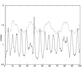
(a)                                              (b)

Figure 2: (a) Nonlinear spectrum and (b) evolution of $U_{max}$ for JONSWAP data ($\gamma=4$ and $\alpha=.016$) that is near homoclinic data. Dashed curve corresponds to 2.2$H_{s}$.

We find that JONSWAP data correspond to “semi-stable” $N$-phase solutions, i.e. we interpret the data as perturbations of $N$-phase solutions with one or more unstable modes (compare Fig. 2(a) with the spectrum of an unstable $N$-phase solution in Fig. 1). In Fig. 2(a) the splitting distance $\delta(\lambda_{+},\lambda_{-})\approx.07$, while in Fig. 3(a) $\delta(\lambda_{+},\lambda_{-})\approx.2$.

        

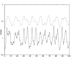
(a)                                              (b)

Figure 3: (a) Nonlinear spectrum and (b) evolution of $U_{max}$ for JONSWAP data ($\gamma=4$ and $\alpha=.016$) that is far from homoclinic data. Dashed curve corresponds to 2.2$H_{s}$.

Thus the JONSWAP data can be quite “near” homoclinic data as in Fig. 2(a) or “far” from homoclinic data as in Fig. 3(a), depending on the values of the phases $\phi_{n}$ in the initial data. For all the examined values of $\alpha$ and $\gamma$ we find that, when $\alpha$ and $\gamma$ are fixed, as the phases in the JONSWAP data vary, the spectral distance $\delta$ of typical JONSWAP data from homoclinic data varies.

Most importantly, irrespective of the values of the JONSWAP parameters $\alpha$ and $\gamma$, in simulations of the NLS equation (1) we find that extreme waves develop for JONSWAP initial data that is “near” NLS homoclinic data, whereas the JONSWAP data that is “far” from NLS homoclinic data typically does not generate extreme waves. Figs. 2(b) and 3(b) show the corresponding evolution of the maximum surface elevation, $U_{max}$, obtained with the NLS equation. $U_{max}$ is given by the solid curve and as a reference, $2.2H_{S}$ (the threshold for a rogue wave) is given by the dashed curve. $H_{S}$ is the significant wave height and is calculated as four times the standard deviation of the wave amplitude. Figure 2(b) shows that when the nonlinear spectrum is near homoclinic data, $U_{max}$ exceeds $2.2H_{S}$ (a rogue wave develops at about $t=40$). Figure 3(b) shows that when the nonlinear spectrum is far from homoclinic data, $U_{max}$ is significantly below $2.2H_{S}$ and a rogue wave does not develop. In this way, we correlate the occurrence of rogue waves characterized by JONSWAP spectrum with the proximity to homoclinic solutions of the NLS equation.

The results of hundreds of simulations of the NLS equation consistently show that proximity to homoclinic data is a crucial indicator of rogue wave events. For example, Fig. 4 shows the synthesis of 200 random simulations of the NLS equation for JONSWAP initial data for different $(\gamma,\alpha)$ pairs (with $\gamma=2,4,6,8,$ and $\alpha=.012,.016$).

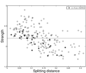
Figure 4: Strength of $U_{max}/H_{s}$ vs. the splitting distance $\delta(\lambda_{+},\lambda_{-})$.

For each such pair $(\gamma,\alpha)$, we performed 25 simulations, each with a different set of randomly generated phases. Each circle represents the strength of the maximum wave ($U_{max}/H_{S}$) attained during one simulation as a function of the splitting distance $\delta(\lambda_{+},\lambda_{-})$. The results for the particular pair $(\gamma=4,\alpha=0.012)$ is represented with an asterisk. A horizontal line at $U_{max}/H_{S}=2.2$ indicates the reference strength for rogue wave formation. We identify two critical values $\delta_{1}=0.08$ and $\delta_{2}=0.22$ that clearly show that (a) if $\delta<\delta_{1}$ (near homoclinic data) rogue waves will occur; (b) if $\delta_{1}<\delta<\delta_{2}$, the likelihood of obtaining rogue waves decreases as $\delta$ increases and, (c) if $\delta>\delta_{2}$ the likelihood of a rogue wave occurring is extremely small.

This behavior is robust. As $\alpha$ and $\gamma$ are varied, the strength of the maximum wave and the occurrence of rogue waves are well predicted by the proximity to homoclinic solutions. The individual plots of the strength vs. $\delta$ for particular pairs $(\gamma,\alpha)$ are qualitatively the same as in Fig. 4 as can be seen by the highlighted case $(\gamma=4,\alpha=0.012)$. These results give strong evidence of the relevance of homoclinic solutions of the NLS equation in investigating rogue wave phenomena for more realistic oceanic conditions and identifies the nonlinear spectral decomposition as a simple diagnostic tool for predicting the occurrence and strength of rogue waves. Finally we remark that the nonlinear spectral analysis can be implemented for other general data (non-JONSWAP) in order to predict the occurrence of rogue waves.

This work was partially supported by NSF Grant No. NSF-DMS0204714.

References

- [1] M. Olagnon and G. Athanassoulis, editors, Rogue waves 2000, volume 32, 2001.
- [2] C. Kharif and E. Pelinovsky, Europ. J. Mech. 22, 603 (2003).
- [3] M. Ablowitz and H. Segur, Solitons and the Inverse Scattering Transform, SIAM, 1981.
- [4] A. Osborne, M. Onorato, and M. Serio, Phys. Lett. A 275, 386 (2000).
- [5] A. Calini and C. Schober, Phys. Lett. A 298, 335 (2002).
- [6] K. Trulsen and K. Dysthe, Wave Motion 24, 281 (1996).
- [7] K. Trulsen, I Kliakhandler,K. Dysthe and M. Velarde Phys. of Fluids 12, 2432 (2000).
- [8] M. Ablowitz, J. Hammack, D. Henderson, and C. Schober, Physica D 152-153, 416 (2001).
- [9] M. Onorato, A. Osborne, M. Serio, and S. Bertone, Phys. Rev. Lett. 86, 5831 (2001).
- [10] N. Ercolani, M.G.Forest, and D. McLaughlin, Physica D 43, 349 (1990).