Chaos suppression in the parametrically driven Lorenz system

Abstract

We predict theoretically and verify experimentally the suppression of chaos in the Lorenz system driven by a high-frequency periodic or stochastic parametric force. We derive the theoretical criteria for chaos suppression and verify that they are in a good agreement with the results of numerical simulations and the experimental data obtained for an analog electronic circuit.

I Introduction

Control of the chaotic dynamics of complex nonlinear systems is one of the most important and rapidly developing topics in applied nonlinear science. In particular, the concept of chaos control, first introduced in Ref. ref_5 , has attracted a great deal of attention over the last decade. Among different methods for controlling chaos that have been suggested by now, the so-called non-feedback control is attractive because of its simplicity: no measurements or extra sensors are required. The idea of this method is to change the complex behavior of a nonlinear stochastic system by applying a properly chosen external force. It is especially advantageous for ultra-fast processes, e.g., at the molecular or atomic level, where no possibility to measure the system variables exists.

Many of the suggested non-feedback methods employ the external forces acting at the system frequencies ref_7 , including parametric perturbations with the frequency that is in resonance with the main driving force. In particular, changing the phase and frequency of a parameter perturbation in a bistable mechanical device was shown to either decrease or increase the threshold of chaos ref_8 . Similarly, unstable periodic orbits are known to be stabilized by a low-frequency modulation of a system control parameter ref_12 , when the control frequency is much lower than the system frequency.

A possibility to change significantly the system dynamics by applying a high- (rather than low- ) frequency force is known for almost a century. As a textbook example, we mention the familiar stabilization of a reverse pendulum (known as the Kapitza pendulum) by rapid vertical oscillations of its pivot ref_13 . This discovery triggered the development of vibrational mechanics ref_14 where the general analysis of nonlinear dynamics in the presence of rapidly varying forces is based on the Krylov-Bogoljubov averaging method ref_15 . In the control theory, the high-frequency forces and parameter modulations are usually used for the vibrational control of non-chaotic nonlinear systems ref_16 . However, as was shown for the example of the Duffing oscillator ref_17 ; ref_exp , chaos suppression can also be achieved by applying a high-frequency parametric force. Later, chaos suppression in the Belousov-Zhabotinsky reaction was demonstrated numerically by adding white noise ref_18 , and the effect of random parametric noise on a periodically driven damped nonlinear oscillator was studied by the Melnikov analysis ref_19 .

In this paper we apply the concepts of the nonresonant non-feedback control to the Lorenz system and demonstrate analytically, numerically, and also experimentally that the suppression of the chaotic dynamics can be achieved by applying a high-frequency parametric or random parametric force. The Lorenz system, found in 1963, is known to produce the canonical chaotic attractor in a simple three-dimensional autonomous system ref_1 ; ref_2 , and it can be applied to describe many interesting nonlinear systems, ranging from thermal convection ref_3 to lasers dynamics ref_4 .

The paper is organized as follows. In Sec. II we present our model and outline the theoretical method and results. By applying the averaging method, we derive the effective Lorenz equations with the renormalized control parameter and obtain the conditions for chaos suppression. In Sec. III, we demonstrate the suppression of chaos by means of direct numerical simulations and also present the experimental data obtained for an analog electronic circuit. Finally, Sec. IV concludes the paper.

II Theoretical approach

II.1 Model

We consider the familiar Lorenz system ref_1 driven by a parametric force. In the dimensionless variables, the nonlinear dynamics is governed by the equations

$$\begin{array}[]{l}{\displaystyle\dot{x}=\sigma(y-x),}\\[9.0pt] {\displaystyle\dot{y}=r[1+f(t)]x-y-xz,}\\[9.0pt] {\displaystyle\dot{z}=xy-bz,}\end{array}$$ (1)

where the dots stand for the derivatives in time, $\sigma$, $r$, and $b$ are the parameters of the Lorenz model, and the function $f(t)$ describes a parametric force. For definiteness but without restrictions of generality, we select the standard set of the parameter values, $\sigma=10$ and $b=8/3$, whereas the parameter $r$ is assumed to vary. It is well known ref_1 that, in the absence of the parametric driving force $f(t)$, the original Lorenz equations demonstrate different dynamical regimes on variation of the control parameter $r$, which are associated with the existence and stability of several equilibrium states. In brief, the system dynamics can be characterized by three regimes:

• the $G_{1}$ regime, for $r<1$: there exists the only stable fixed point at the origin, $(x,y,z)=(0,0,0)$;

• the $G_{2}$ regime, for $1<r<24.74$: the origin becomes unstable, two new fixed points appear, $(x,y,z)=(\pm\sqrt{b(r-1)},\pm\sqrt{b(r-1)}/r,r-1)$;

• the $G_{3}$ regime, for $r>24.74$: no stable fixed points exist, chaotic dynamics occur with a strange attractor.

We consider the special case of the general model (1), assuming that the characteristic frequency of the parametric force $f(t)$ is much larger than the characteristic frequency of the unforced Lorenz system, where the frequency (which is the mean-time derivative of the phase) of the Lorenz system can be defined as ref_10

$$\omega_{0}=\lim_{T\rightarrow\infty}\frac{2\pi N(T)}{T},$$ (2)

where $N(T)$ is the number of turns performed in $T$.

II.2 Periodic driving force

First, we consider the case of a periodic driving force,

$$f(t)=k\cos(\omega t).$$ (3)

Assuming that the frequency of parametric modulations is large ($\omega\gg\omega_{0}$), we apply an asymptotic analytical method ref_13 ; ref_14 based on a separation of different time scales, and derive the effective equations that describe the slowly varying dynamics. To do this, we decompose every variable into a sum of slowly and rapidly varying parts, i.e.,

$$x=X+\xi,\;y=Y+\eta,\;z=Z+\zeta,$$ (4)

where the functions $\xi(t)$, $\eta(t)$, and $\zeta(t)$ describe fast oscillations around the slowly varying envelope functions $X(t)$, $Y(t)$, and $Z(t)$, respectively. The rapidly oscillating corrections are assumed to be small in comparison with the slowly varying parts, and their mean values during an oscillation period vanish, i.e. $<x>=X$, $<y>=Y$, and $<z>=Z$. Substituting the Eq. (4) into Eq. (1) with the force (3), and averaging over the oscillation period, we obtain the following equation,

$$\begin{array}[]{l}{\displaystyle\dot{X}=\sigma(Y-X),}\\[9.0pt] {\displaystyle\dot{Y}=rX-Y-XZ+rk<\xi\cos(\omega t)>,}\\[9.0pt] {\displaystyle\dot{Z}=XY-bZ,}\end{array}$$ (5)

where the terms $<\xi\zeta>$ and $<\xi\eta>$ are neglected because, for large $\omega$, they are all of the higher orders in $k\omega^{-1}$. Using Eq. (5) and keeping only the terms not smaller than those of the order of $k\omega^{-1}$ and $k$, respectively, we find the equations, $\dot{\xi}=\sigma\eta$ and $\dot{\eta}=rkX\cos(\omega t)$. Regarding the function $X$ as constant during the period of the function $f(t)$, we obtain the solution $\xi=-\sigma r(k/\omega^{2})X\cos(\omega t)$, and thus $<\xi\cos(\omega t)>=-\sigma r(k/2\omega^{2})X$. Therefore, the averaged equations (5) are

$$\begin{array}[]{l}{\displaystyle\dot{X}=\sigma(Y-X),}\\[9.0pt] {\displaystyle\dot{Y}=r_{\rm eff}X-Y-XZ,}\\[9.0pt] {\displaystyle\dot{Z}=XY-bZ,}\end{array}$$ (6)

where

$$r_{\rm eff}=r(1-rK_{\omega}),\;\;\;\;K_{\omega}=\frac{\sigma k^{2}}{2\omega^{2}}>0.$$ (7)

As a result, the averaged dynamics of the Lorenz system in the presence of a rapidly varying parametric force is described by the effective renormalized Lorenz equations (6) with the effective control parameter $r_{\rm eff}$, so that all dynamical regimes and the route to chaos discussed earlier can be applicable directly to Eq. (6), assuming the effect of the renormalization.

Therefore, in terms of the averaged system, for $r_{\rm eff}\leq 1$, i.e. under the condition

$$K_{\omega}\geq(r-1)/r^{2},$$ (8)

the fixed point at the origin remains stable and, therefore, in terms of the original Lorenz system, the chaotic dynamics should be suppressed. Next, for $1<r_{\rm eff}\leq 24.74$, i.e. under the condition

$$(r-24.74)/r^{2}\leq K_{\omega}<(r-1)/r^{2},$$ (9)

the Lorenz chaos is also suppressed and the stable saddle-focus points appears: $X_{0}=Y_{0}=\pm\sqrt{b(r_{\rm eff}-1)}$, $Z_{0}=r_{\rm eff}-1$.

Relations (8) and (9) that follow from the averaged equations, define the conditions for the chaos suppression; they can be expressed as relations between the amplitude and frequency of the rapidly varying oscillations,

$$k\geq\omega\sqrt{2(r-1)/\sigma r^{2}},$$ (10)

$$\omega\sqrt{2(r-24.7)/\sigma r^{2}}\leq k<\omega\sqrt{2(r-1)\sigma r^{2}}.$$ (11)

The dependencies $K_{\omega}\sim r$ (see Eqs. (8) and (9)) and $k\sim\omega$ (see Eqs. (10) and (11)) are the key characteristics of the chaos suppression effect that we verify numerically and compare with the experimental data obtained with an analog electronic circuit (see Figs. 4 and 5 below).

II.3 Random driving force

Now we turn to the case of a random force, and treat the function $f(t)$ in Eq. (1) as random by formally writing $f(t)=\epsilon(t)$, where $\epsilon(t)$ describes a bandwidth-limited noise with a power spectral density

$$P_{\epsilon}(\omega)=\Biggr{\{}\begin{array}[]{l}{\displaystyle p(\omega),\,\;\;{\rm when}\;\omega_{1}<|\omega|<\omega_{2},}\\[9.0pt] {\displaystyle 0,\,\;\;{\rm when}\;|\omega|<\omega_{1},|\omega|>\omega_{2},}\end{array}$$ (12)

and the zero mean value, $<\epsilon(t)>=0$. In order to apply the analytical method discussed above, the noise $\epsilon(t)$ is assumed to be composed of high-frequency components only, i.e. $\tilde{\omega}\gg\omega_{0}$, where

$$\tilde{\omega}=\int^{\infty}_{-\infty}\omega P_{\epsilon}(\omega)d\omega\left[\int^{\infty}_{-\infty}P_{\epsilon}(\omega)d\omega\right]^{-1}$$

is the characteristic frequency of the bandwidth-limited parametric fluctuations. Again, decomposing the system variables into sums of slow and rapidly varying functions and averaging over the period $T_{0}$, we obtain

$$\begin{array}[]{l}{\displaystyle\dot{X}=\sigma(Y-X),}\\[9.0pt] {\displaystyle\dot{Y}=rX-Y-XZ+rk<\xi(t)\epsilon(t)>,}\\[9.0pt] {\displaystyle\dot{Z}=XY-bZ,}\end{array}$$ (13)

where the value of $T_{0}$ is much smaller than the characteristic time scale of the Lorenz system oscillations but sufficiently larger than the time scale of fluctuations, i.e. $2\pi/\tilde{\omega}<T_{0}\ll 2\pi/\omega_{0}$. Then, the equations for the rapid parts can be reduced to the equations, $\dot{\xi}=\sigma\eta(t)$ and $\dot{\eta}=r\epsilon(t)X$. Thus, the key averaged quantity becomes $<\xi(t)\epsilon(t)>=<\xi(t)\ddot{\xi}(t)>/(\sigma rX)$. On the other hand, for the stationary random process $\xi(t)$, the following expressions are valid,

$$<\xi(t)\ddot{\xi(t)}>=-<\dot{\xi}^{2}(t)>=-\int^{\infty}_{-\infty}\omega^{2}P_{\xi}(\omega)d\omega,$$

where $P_{\xi}(\omega)=|H(\omega)|^{2}P_{\epsilon}(\omega)$ is the power spectral density of $\xi(t)$ and $H(\omega)=-\sigma rX/\omega^{2}$ is the frequency response function for the equation $\ddot{\xi}=\sigma rX\epsilon(t)$. As a result, we obtain the averaged equations in the form (6) where this time [cf. Eq. (7)]

$$r_{\rm eff}=r(1-rK_{\epsilon}),\;\;\;K_{\epsilon}=2\sigma\int^{\omega_{2}}_{\omega_{1}}\frac{p(\omega)}{\omega^{2}}d\omega.$$ (14)

The quantity $K_{\epsilon}$ is related to the intensity of the parametric fluctuations $\epsilon(t)$ and it is always positive. Since the averaged equations have the same form as the original unforced Lorenz equations but with the effective control parameter $r_{\rm eff}$ instead of $r$, there appears the parameter region where the chaotic dynamics is suppressed. In particular, for $r_{\rm eff}\leq 1$, i.e., under the condition

$$K_{\epsilon}\geq(r-1)/r^{2},$$ (15)

the fixed point at the origin remains stable in the presence of rapidly varying fluctuations. When $1<r_{\rm eff}\leq 24.74$, i.e. for

$$(r-24.74)/r^{2}\leq K_{\epsilon}<(r-1)/r^{2},$$ (16)

two new saddle-focus fixed points appear, with the coordinates $X_{0}=Y_{0}=\pm\sqrt{b(r_{\rm eff}-1)}$, $Z_{0}=r_{\rm eff}-1$.

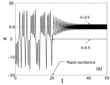
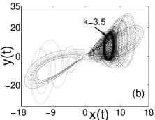
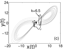
Figure 1: (a) Numerical simulation of chaos suppression shown for the evolution of the function $x(t)$. The high-frequency parametric force is turned on at the point $t=20$, and it moves the system to a new fixed point $<x(t)>=6.8$, for $k=3.5$, or it stabilizes the origin $x(t)=0$, for $k=6.5$. (b,c) Phase plane representation of the system dynamics for (b) $k=3.5$ and (c) $k=6.5$.

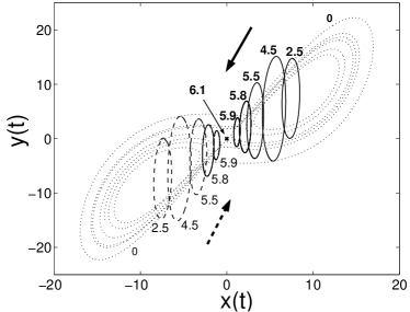
Figure 2: Phase plane representation of the system dynamics after the suppression of chaos, at different values of the parametric force amplitude (marked in the figure).

When the random function $\epsilon(t)$ describes a bandwidth-limited white noise, $P_{\epsilon}(\omega)=S_{0}$, the renormalization factor $K_{\epsilon}$ can be written as

$$K_{\epsilon}=\frac{2\sigma(\omega_{2}-\omega_{1})}{\omega_{1}\omega_{2}}S_{0}=\frac{\sigma<\epsilon^{2}(t)>}{\omega_{1}\omega_{2}},$$ (17)

and the effective control parameter is simplified to be

$$r_{\rm eff}=r\left(1-\frac{\sigma r}{\omega_{1}\omega_{2}}<\epsilon^{2}(t)>\right),$$ (18)

so that the chaos suppression effect is clearly proportional to the noise intensity. Moreover, in the limit $\omega_{1},\omega_{2}\rightarrow\omega$, we recover the result $K_{\epsilon}=\sigma k^{2}/(2\omega^{2})$ obtained earlier for the periodic parametric force [see Eq. (7)].

III Numerical simulations and experimental results

To verify out theory, first we perform direct numerical simulations of the full model (1). Figures 1 and 2 show the results for the system temporal evolution obtained numerically by solving Eqs. (1) and (3) with the parameters: $(\sigma,b,r)=(10,8/3,28)$. Since the mean frequency of the unforced oscillations of the Lorenz system is found to be $\omega_{0}=8.24$ [see Eq. (2)], for the above parameters the frequency of the rapid parametric force is chosen as $\omega=70$. As shown in the examples presented in Fig. 1, the fixed point at the origin $x=0$ is stabilized for $k=6.5$ whereas a new stationary point $X_{0}=6.8$ appears for $k=3.5$. We can see from Fig. 2 that the system dynamics in the phase space after the suppression of chaos is reduced to the coexisting limit cycles (marked in solid and dotted) whose averaged behavior is described by Eq. (6), shrinking to the origin as the parametric force amplitude $k$ is increased.

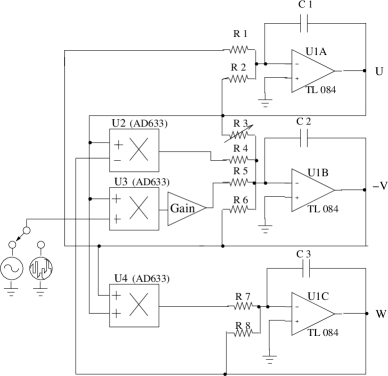
Figure 3: Schematic of the analog electric circuit representing the Lorenz oscillator in the rescaled variables, including the parametric driving force and fluctuations.

Next, we study experimentally the chaos suppression in the Lorenz system in the framework of an analog electronic circuit implementation of the Lorenz system (see, e.g., Refs. cuomo ; kurths ). Our circuit uses three Op-Amps (TL084) as the building blocks for the operations of sum, difference, and integration, and three analog multipliers (AD633) for the operations of product.

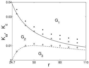
Figure 4: Experimental vs. theoretical results shown as the stability regions in the parameter plane ($K_{\omega}$/$K_{\epsilon}$, $r$). Solid: theoretical result [Eq. (8) and Eq.(15)] for stabilization of the fixed point at the origin. Dashed: the theoretical results (9) and (16) for the transition to a new oscillating state. Squares and diamonds: experimental results for the periodic driving force with the frequency $\omega=1$KHz. Asterisks: the critical values $K_{\epsilon}$ for the chaos suppression by a bandwidth-limited white noise with $\omega_{1}=700$Hz and $\omega_{2}=1300$Hz.

As the first step, we rescale the variables $x$, $y$, and $z$ in order to fit within the dynamical range of the source (-15V, 15V), and such that the circuit operates in the frequency range of a few kHz. Applying the transformations $u=x/10$, $v=y/10$, $w=z/10$, and $\tau=t/A$, we obtain the rescaled Lorenz system, where $\omega^{\prime}=A\omega$, so that $\omega t=\omega^{\prime}\tau$ ($\tau$ is measured in seconds). The rescaled equations describe the temporal evolution of the corresponding output voltages of Op-Amps in the analog electronic circuit, as shown schematically in Fig. 3.

In the electric circuit shown in Fig. 3, the analog multipliers (AD633) have a noticeable offset at the output that may alter the dynamical behavior of the system; this effect has been compensated by using a compensation array. The parameters of the Lorenz model can be defined through the values of the resistors, $\sigma=R_{6}/R_{1}=R_{6}/R_{2}$, $b=R_{6}/R_{8}$, $r=R_{6}/R_{3}$, and the values of the resistors used are: $R_{1}=R_{2}=100k\Omega$, $R_{3}=35.7k\Omega$ (for $r=28$), $R_{4}=R_{7}=10k\Omega$, $R_{5}=5k\Omega$, and $R_{8}=374k\Omega$, whereas the values of the capacitors are: $C_{1}=C_{2}=C_{3}=C=100nF$. The tolerance of the resistors and capacitors is less than 1%. For these values, the parameters take the following values: $\sigma=10$, $b=2.67$, and $A=1/R_{6}C=10(s^{-1})$. The control parameter $r$ of the Lorenz system and the force amplitude $k$ can be adjusted by varying the resistor $R_{3}$ through the relation $r=10^{6}\Omega/R_{3}$ and changing the amplification coefficient of the gain-block element, respectively, as shown in Fig. 3. In the electric circuit, the frequency of the unforced oscillations for $r=28$ is found to be $\omega_{0}^{\prime}=A\omega_{0}=13.1$Hz$=82.4$ rad/s. Therefore, we apply a parametric force with the frequency larger than 65Hz.

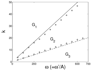
Figure 5: Experimental vs. theoretical results for the critical amplitude of the parametric force vs. frequency for $r=28$. Analytical results (10) and (11) are plotted as solid and dashed lines, respectively. Squares and diamonds show the experimental results for the stabilization of the origin and the suppression of chaos into a fixed point, respectively.

Figure 4 shows the threshold curves described by Eqs. (8) and (9), as well as Eqs. (15) and (16) that define three regions with different nonlinear dynamics, as compared with the numerical and experimental data. The domains $G_{1}$ and $G_{2}$ indicate the regions for stabilizing the fixed point at the origin and the transition to a new fixed point, respectively, whereas the domain $G_{3}$ is the region of the chaotic dynamics. The critical values of $K_{\omega}$ were obtained experimentally by changing the amplitude $k$ of the parametric driving force at the fixed frequency $\omega=1$kHz, the corresponding experimental data are presented in Fig. 4 by squares and diamonds. In the experiment with parametric fluctuations (the data are marked by asterisks), bandwidth-limited white noise with the limits $\omega_{1}=700$Hz and $\omega_{2}=1300$Hz was applied, and its strength was adjusted by gain-block element (Fig. 3).

Figure 5 shows the dependence of the critical amplitude of the parametric force for the chaos suppression as a function of the frequency. Solid and dashed lines represent the theoretical results described by Eq. (10) and Eq. (11), respectively, whereas the experimental data are plotted as squares and diamonds. As shown in Fig. 4 and Fig. 5, the experimental results are in a good agreement with the theoretically calculated threshold dependencies.

IV Conclusions

We have studied analytically, numerically, and experimentally the suppression of chaos in the Lorenz system driven by a rapidly oscillating periodic or random parametric force. We have derived the theoretical criteria for chaos suppression which indicate that, for a fixed value of the control parameter $r$, the critical amplitude of the force required for the suppression of chaos is proportional to its frequency. The theoretical criteria for chaos suppression have been found to agree well with both the results of numerical simulations and the experimental data obtained for an analog electronic circuit.

C.-U.C. and Y.S.K thank the Alexander von Humboldt Stiftung for research scholarships. The work was also supported by the Deutsche Forschungsgemeinschaft.

References

- (1) E. Ott, C. Grebogi, and J.A. Yorke, Phys. Rev. Lett. 64, 1196 (1990).
- (2) R. Lima and M. Pettini, Phys. Rev. A 41, 726 (1990); Y. Braiman and I. Goldhirsch, Phys. Rev. Lett. 66,2545 (1991); L. Fronzoni, M. Giocondo, and M. Pettini, Phys. Rev. A 43, 6483 (1991); R. Chacón and J. Díaz Bejarano, Phys. Rev. Lett. 71, 3103 (1993); R. Lima and M. Pettini, Int. J. Bifurcation and Chaos 8, 1675 (1998).
- (3) L. Fronzoni and M. Giocondo, Int. J. Bifurcation and Chaos 8, 1693 (1998).
- (4) R. Vilaseca, A. Kul’minskii, and R. Corbalán, Phys. Rev. E 54, 82 (1996); R. Dykstra et al., Phys. Rev. E 57, 397 (1998); A.N. Pisarchik, B.F. Kuntsevich, and R. Corbalán, Phys. Rev. E 57, 4046 (1998); A.N. Pisarchik and R. Corbalán, Phys. Rev. E 59, 1669 (1999).
- (5) L.D. Landau and M. Lifshitz, Mechanics (Pergamon Press, Oxford, 1960).
- (6) I. Blekhman, Vibrational Mechanics (World Scientific, Singapore, 2000).
- (7) N.N. Bogoljubov and Yu.A. Mitropolski, Asymptotic Methods in the Theory of Nonlinear Oscillations (Gordon and Breach, New-York, 1961).
- (8) G. Zames and N.A. Shneydor, IEEE Trans. Aut. Contr. AC-21, 660 (1976); R. Bellman, J. Bentsman, and S. Meerkov, IEEE Trans. Aut. Contr. AC-31, 710 (1986).
- (9) Yu.S. Kivshar, F. Rödelsperger, and H. Benner, Phys. Rev. E 49, 319 (1994).
- (10) F. Rödelsperger, Yu.S. Kivshar, and H. Benner, J. Magn. Magn. Mat. 140-144, 1953 (1995).
- (11) K. Matsumoto and I. Tsyda, J. Stat. Phys. 31, 87 (1983).
- (12) V. Basios, T. Bountis, and G. Nicolis, Phys. Lett. A 251, 250 (1999).
- (13) E.N. Lorenz, J. Atmos. Sci. 20, 131 (1963).
- (14) I. Stewart, Nature 406, 948 (2000).
- (15) See, e.g., H.G. Schuster, Deterministic Chaos (VCH Weinheim, 1984).
- (16) M.Y. Li, Tin Win, C.O. Weiss, and N.R. Heckenberg, Opt. Commun. 80, 119 (1990)
- (17) E.-H. Park, M.A. Zaks, and J. Kurths, Phys. Rev. E 60, 6627 (1999).
- (18) K.M. Cuomo and A.V. Oppenheim, Phys. Rev. Lett. 71, 65 (1993).
- (19) A. Pujol-Peré, O. Calvo, M.A. Matías, and J. Kurths, Chaos 13, 319 (2003).