Coupled-mode theory for spatial gap solitons in optically-induced lattices

Abstract

We develop a coupled-mode theory for spatial gap solitons in the one-dimensional photonic lattices induced by interfering optical beams in a nonlinear photorefractive crystal. We derive a novel system of coupled-mode equations for two counter-propagating probe waves, and find its analytical solutions for stationary gap solitons. We also predict the existence of moving (or tilted) gap solitons and study numerically soliton collisions.

It is well known that a periodic modulation of the optical refractive index not only modifies the spectrum of linear waves, but also strongly affects nonlinear propagation and self-trapping of light book0 ; book . Recently, formation of spatial solitons in reconfigurable photonic lattices in photorefractive materials has been demonstrated experimentally in one- Fleischer:2003-23902:PRL ; Neshev:2003-710:OL and two- Fleischer:2003-147:Nature dimensional geometries. In this case, strong electro-optic anisotropy of a photorefractive crystal was employed to create the lattice by interfering laser beams with ordinary polarization, while the solitons were observed in the orthogonally polarized mode.

Periodically modulated nonlinear systems can also support self-trapped localized pulses or beams in the form of gap solitons (GSs), which are hosted by a gap of the system’s linear spectrum, induced by the resonant Bragg coupling between the forward- and backward-propagating waves deSterke . A notable property of the GSs are that they can form in both self-focusing and self-defocusing media.

Travelling temporal-domain GSs have been observed experimentally in material Bragg gratings written in silica fibers Eggleton:1996-1627:PRL . The concept of a spatial-domain GS was proposed Feng ; Nabiev and further elaborated in waveguide settings kivshar ; Mak-spatial ; sukhorukov . Experimentally, spatial GSs were demonstrated in waveguide arrays Mandelik and optically-induced photonic lattices gap_induced .

The simplest and most ubiquitous description of the GSs is provided by the coupled-mode theory (CMT), which amounts to the derivation of a system of coupled nonlinear propagation equations for the forward and backward waves deSterke . In this Letter, we derive a novel type of the CMT model for spatial GSs in the optically-induced photonic lattice. We find exact analytical solutions for GSs in the framework of this model, and compare them with the results obtained numerically by solving the full nonlinear model. We thus identify a parameter region where the couple-mode approximation is accurate enough, and in that region we use the model to predict new features such the existence of the families of moving (or tilted) gap solitons and to study their interaction Actually, the new model derived in this work may have more general purport than just an asymptotic approximation for the nonlinear photonic lattice, as it is the first coupled-mode system that accounts for a saturable nonlinearity.

Following Refs. Fleischer:2003-23902:PRL ; Neshev:2003-710:OL , we consider the evolution of an extraordinarily polarized probe beam propagating through a periodic structure written by counter-propagating ordinary-polarized plane-wave beams in the photorefractive medium. As mentioned above, the electro-optic coefficients in the crystal are substantially different for the orthogonal polarizations, therefore the grating, created by interference of the counter-propagating beams, is essentially one-dimensional (uniform along the propagation axis $z$). The interference of the plane waves with a wavelength $\lambda$ creates an intensity distribution, $I_{g}(x)=I_{0}\cos^{2}(Kx)$, with $K=2\pi n_{0}\lambda^{-1}\sin\theta$, where $\theta$ is the angle between the Poynting vectors of the plane waves and the $z$ axis, and $n_{0}$ is the refractive index along the ordinary axis. Provided that the intensity of the probe beam, $|E|^{2}$, is much weaker than that of the grating, $I_{0}$, one may neglect the feedback action of the probe beam on the grating (a perturbative calculation within the framework of an extended model, that includes equations for both the lattice-forming and probe fields, shows that the feedback exactly cancels out at the first order in $1/I_{0}$). Then the evolution of the local amplitude $E(x,z)$ of the probe beam obeys the known equation Fleischer:2003-23902:PRL ; Neshev:2003-710:OL , whose normalized form is

$$i\frac{\partial E}{\partial z}+\frac{1}{2}\frac{\partial^{2}E}{\partial x^{2}}-\frac{E}{1+I_{0}\cos^{2}(Kx)+|E|^{2}}=0.$$ (1)

To derive the corresponding equations for the coupled forward and backward waves, we approximate solutions to Eq. (1) by

$$E(x,z)=u(x,z)e^{iKx}+v(x,z)e^{-iKx},$$ (2)

where $u$ and $v$ are slowly varying [in comparison with the carrier waves $\exp\left(\pm iKx\right)$] envelopes of the forward and backward modes. Substituting the expansion (2) into Eq. (1), we perform the Fourier expansion with respect to $\exp\left(\pm iKx\right)$ and, in the spirit of the CMT approach, keep only the lowest-order harmonics. Eventually, this leads to the following CMT equations (one of which is linear):

$$i\frac{\partial}{\partial z}(u-v)+iK\frac{\partial}{\partial x}(u+v)$$

$$-\frac{2(u-v)}{\sqrt{I_{0}(1+|u-v|^{2})+1+2\left(|u|^{2}+|v|^{2}\right)}}=0,$$ (3)

$$i\frac{\partial}{\partial z}(u+v)+iK\frac{\partial}{\partial x}(u-v)=0.$$ (4)

Equations (3) and (4) constitute a new CMT model with the saturable nonlinearity. It contains one irreducible parameter $I_{0}$, while $K$ can be absorbed by rescaling of $x$.

In the physically relevant case, the photonic-lattice intensity is large, i.e., $I_{0}\gg 1,|u|^{2},|v|^{2}$, hence the square root in Eq. (3) may be approximated by $\sqrt{I_{0}(1+|u-v|^{2})}$, except for a vicinity of point(s) where $w\equiv u-v$ vanishes. Using this approximation, and eliminating $\left(u+v\right)$ by means of Eq. (4), we reduce Eq. (3) to an equation for the single function $w$,

$$\frac{\partial^{2}w}{\partial z^{2}}-K^{2}\frac{\partial^{2}w}{\partial x^{2}}+\frac{2i}{\sqrt{I_{0}}}\frac{\partial}{\partial z}\left(\frac{w}{\sqrt{(1+|w|^{2})}}\right)=0.$$ (5)

We have checked the accuracy of the simplified equation (5), comparing its analytical solutions for solitons (see below), and their stability, vs. direct numerical solutions of Eqs. (3) and (4). A conspicuous difference appears only in the region of $I_{0}\,{}_{\sim}^{<}\,3$, where the CMT does not provide for an adequate approximation anyway.

Stationary solutions of Eq. (5) are sought for as $w(x,z)=e^{iqz}W(x)$, where a real function $W$ obeys the equation $d^{2}W/dx^{2}=-dU_{\mathrm{eff}}/dW$, with

$$U_{\mathrm{eff}}(W)=\frac{q^{2}}{2K^{2}}W^{2}+\frac{2q}{K^{2}\sqrt{I_{0}}}\left(\sqrt{1+W^{2}}-1\right).$$ (6)

Further, Eq. (4) shows that, for the stationary solutions,

$$(u,v)=\frac{1}{2}e^{iqz}\left[W(x)\pm\frac{iK}{q}\frac{dW}{dx}\right].$$ (7)

If the propagation constant $q$ belongs to the interval (which is, actually, the bandgap)

$$0<-q<2{\Large/}\sqrt{I_{0}}\equiv Q,$$ (8)

the potential (6) has two symmetric minima, giving rise to GS solutions that can be written in an implicit analytical form,

$$\left(KW^{\prime}\right)^{2}=-\left(qW\right)^{2}+\left(4|q|{\Large/}\sqrt{I_{0}}\right)\left(\sqrt{1+W^{2}}-1\right).$$ (9)

As it follows from Eq. (9), the soliton’s squared amplitude is $W_{\mathrm{max}}^{2}=(8/q^{2}I_{0})(2-\sqrt{I_{0}}|q|)$. In the small-amplitude limit, i.e., for $0<\epsilon\equiv 2(2-|q|\sqrt{I_{0}})\ll 1$ [cf. Eq. (8)], the GS asymptotically coincides with the conventional nonlinear-Schrödinger soliton, $W(x)=\pm\sqrt{\epsilon}\;\mathrm{sech}\left(\sqrt{\epsilon|q|/2}K^{-1}I_{0}^{-1/4}x\right)$. In the other limit, $|q|\rightarrow 0$, the soliton assumes a “compacton” shape: $|q|\sqrt{I_{0}}W(x)=4\cos^{2}\left(|q|K^{-1}I_{0}^{-1/4}x\right)$, if $|x|<\pi KI_{0}^{1/4}/\left(2|q|\right)$, and $W(x)=0$ otherwise. However, the conditions under which the CMT equations were derived above do not hold in the latter case.

To verify the validity of the CMT approximation in the present setting, in Fig. 1 we compare the analytical soliton solutions based on Eq. (9) and ones found numerically from Eq. (1). The comparison is presented in terms of a global characteristic of the soliton family, viz., the integral power, $N=\int_{-\infty}^{+\infty}|E(x)|^{2}dx$, vs. the propagation constant $q$; an example of the comparison of the soliton’s shapes is also included. Naturally, the approximation is appropriate sufficiently close to the gap’s edge. We also note that the negative slope of the $N(q)$ dependence suggests stability of the entire soliton family as per the Vakhitov-Kolokolov criterion, i.e., the absence of real eigenvalues in the spectrum of small perturbations around the soliton VK . However, the solitons may be subject to instabilities with complex eigenvalues. Detailed numerical analysis shows that, in the case of large $I_{0}$, when the the CMT approximation is relevant, a stable part of the soliton family in the bandgap (8) is limited to a sub-gap,

$$Q-\Delta Q<-q<Q.$$ (10)

The width of the stability sub-gap, $\Delta Q\approx 0.21$, is nearly constant for $I_{0}\,{}_{\sim}^{>}\,20$ [for $I_{0}=25.5$, which is the case shown in Fig. 1, the GSs are stable in $\approx 53\%$ of the interval (8); we mention, for comparison, that in the standard GS model with the cubic nonlinearity, the stable part occupies $\approx 51\%$ of the bandgap is Rich ; CapeTown ]. Unstable solitons [which actually occupy that part of the bandgap (8) where the CMT approximation is irrelevant] are destroyed by perturbations.

The CMT approximation opens many ways to investigate novel phenomena which may be difficult to study directly within the framework of the full model. An issue of obvious interest are moving (or tilted) GSs, of the form $\left(u,v\right)=e^{iqz}\left(U(x-cz),V(x-cz)\right)$. Our analysis shows that the bandgap (8) for the tilted solitons shrinks to $0<-q<\tilde{Q}\equiv Q\sqrt{1-(c/K)^{2}}$, and it does not exist for $c^{2}>K^{2}$. The reduced gap is completely filled with moving gap solitons which are stable in the sub-gap $\tilde{Q}-\Delta Q<-q<\tilde{Q}$, cf. Eq. (10), with the width $\Delta Q$ that does not depend on the tilt $c$, up to the accuracy of numerical results (the latter fact resembles a known stability feature of the GSs in the conventional CMT approach CapeTown ).

The stability of the tilted solitons suggests to consider collisions (intersections) between them. The most important characteristic of soliton interactions is elasticity. Our numerical simulations demonstrate that the interaction is quite elastic, unless the solitons are taken close to the instability border [which is $-q=Q-\Delta Q$, see Eq. (10)]. In the latter case, there is a specific structure of regions of elastic and inelastic collisions in the plane $\left(c_{1},-c_{2}\right)$ of the tilts of two colliding solitons, as shown in Fig. 2. In the case of inelasticity, the colliding solitons suffer strong perturbations.

In conclusion, we have developed the coupled-mode theory for spatial gap solitons in one-dimensional photonic lattices written optically in a photorefractive medium. We have derived a novel type of the coupled-mode equations and found their analytical solutions for gap solitons. In the case when the coupled-mode system correctly approximates the photonic lattice, we used the model to investigate new features of such systems, such as the existence and stability of moving gap solitons and their collisions. The latter results suggest new experiments for optically-induced lattices in photorefractive media.

This work was partially supported by the Australian Research Council. B.A.M. appreciates hospitality of the Nonlinear Physics Center at the Australian National University.

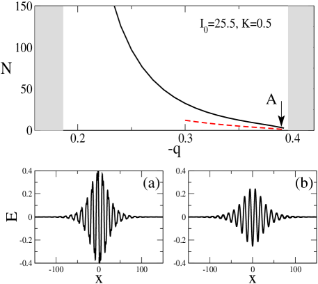
Figure 1: The integral power of the soliton vs. the propagation constant [in the first finite gap of Eq. (1)] at $I_{0}=25.5$ and $K=0.5$ . The solid and dashed lines show, respectively, the numerical result, and the analytical one, as obtained from Eqs. (9), (7), and (2). Examples of numerical (a) and analytical (b) profiles of a soliton taken close to the edge of the gap ($q=0.39$, point A) are shown in the bottom part of the figure.

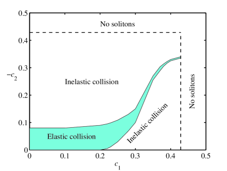
Figure 2: Regions of elastic and inelastic head-on collisions between two solitons, with the tilts $c_{1}>0$ and $c_{2}<0$, and $|q_{1}|=|q_{2}|=0.2$ (close to the instability border, which is $|q|=Q-\Delta Q\approx 0.19$, in this case), at $I_{0}=25.5$ and $K=0.5$.

References

- (1) R. E. Slusher and B. J. Eggleton, Eds., Nonlinear Photonic Crystals, Springer Series in Photonics, Vol. 10 (Springer-Verlag, Berlin, 2003), 375 pp.
- (2) Yu. S. Kivshar and G. P. Agrawal, Optical Solitons: From Fibers to Photonic Crystals (Academic, San Diego, 2003), 560 pp.
- (3) J. W. Fleischer, T. Carmon, M. Segev, N. K. Efremidis, and D. N. Christodoulides, Phys. Rev. Lett.90, 023902 (2003).
- (4) D. Neshev, E. A. Ostrovskaya, Yu. S. Kivshar, and W. Krolikowski, Opt. Lett. 28, 710 (2003).
- (5) J. W. Fleischer, M. Segev, N. K. Efremidis, and D. N. Christodoulides, Nature 422, 147 (2003).
- (6) C. M. de Sterke and J. E. Sipe, in Progress in Optics, Vol. XXXIII, Ed. E. Wolf (North-Holland, Amsterdam, 1994), p. 203.
- (7) B. J. Eggleton, R. R. Slusher, C. M. de Sterke, P. A. Krug, and J. E. Sipe, Phys. Rev. Lett. 76, 1627 (1996).
- (8) J. Feng, Opt. Lett. 18, 1302 (1993).
- (9) R. F. Nabiev, P. Yeh, and D. Botez, Opt. Lett. 18, 1612 (1993).
- (10) Yu.S. Kivshar, Phys. Rev. E 51, 1613 (1995).
- (11) W. C. K. Mak, B.A. Malomed, and P. L. Chu, Phys. Rev. E 58, 6708 (1998).
- (12) A. A. Sukhorukov and Yu. S. Kivshar, Opt. Lett. 27, 2112 (2002).
- (13) D. Mandelik, R. Morandotti, J. S. Aitchison, and Y. Silberberg, Phys. Rev. Lett. 92, 093904 (2004).
- (14) D. Neshev, A. A. Sukhorukov, B. Hanna, W. Krolikowski, and Yu. S. Kivshar, Phys. Rev. Lett. 93, 083905 (2004).
- (15) M. G. Vakhitov and A. A. Kolokolov, Radiophys. Quantum Electron. 16, 783 (1973).
- (16) B. A. Malomed and R. S. Tasgal, Phys. Rev. E 49, 5787 (1994).
- (17) I. V. Barashenkov, D. E. Pelinovsky, and E. V. Zemlyanaya, Phys. Rev. Lett. 80, 5117 (1998).