[nlin/0411019] Large-Scale Coherence and Law of Decay of Two-Dimensional Turbulence

Two-dimensional (2D) turbulence is a simplified system mimicking such important phenomena, as ubiquitous vortex generation, in atmospheric flows. The vortex formation as a dominant process of 2D hydrodynamics has been recognized by Onsager more than half a century ago¹ and, thanks to obsession of TV stations with the weather forcast, the relevance of spontanious emergence of strong vortices out of quiescent background for the world we live in, can be verified at any time of the day. Many features of the vortex formation in decaying 2D turbulence have been undestood due to numerical and theoretical works of McWilliams and collaborators^2-5, Benzi et. al.⁶ and many others. Still, many new features have recently been discovered and some important questions remained unanswered.

The problem of decay of two-dimensional (2D) turbulence considered in our recent paper⁷ and the one, we are interested in here, is formulated in a following way. Consider a time evolution of an initial velocity field, $u(x,y,0)={\bf u}_{0}$ defined on a two-dimensional square such that $-L\leq x,y\leq L$ . The field $u_{0}$ is a Gaussian random noise supported in the Fourier space in the vicinity of $k=k_{0}(t=0)=O(\frac{N\pi}{L})$ with $\overline{{\bf u}^{2}_{0}}=O(1)$ and $N=const=O(1)$ . At the initial instant, $t=0$ , the enstrophy is $\Omega=\overline{\omega^{2}}\equiv\omega_{0}^{2}=\overline{(\nabla\times{\bf u})^{2}}=O(1)$ . The square is large meaning that we are interested in the limit $\nu\rightarrow 0$ and $k_{0}(t=0)L\rightarrow\infty$ . Still, the box is finite so we will be able to study both short time, when $k_{0}(t)L\gg 1$ , and long time asymptotics when $k_{0}(t)L\approx 1$ . In all our simulations the initial kinetic energy of the flow $K(t=0)=\frac{1}{2}\rho\int v^{2}({\bf x},t=0)d{\bf x}=\frac{1}{2}$ and the fluid density $\rho=1$ . This set up with the basically structureless initial field is ideal for investigation of the details of the structure emergence in the course of the flow evolution.

According to a recent theory⁸, in an infinite system ( $L\rightarrow\infty$ ), the universal asymptotic law of enstrophy decay is $\Omega\propto t^{-\gamma}$ with $\gamma={\frac{2}{3}}$ which is close to the short -time results of simulation by Chasnov⁹ ( $\gamma\approx 0.7-0.8$ ) and our own⁷ $\gamma\approx 0.7$ . At the later times, after the large-scale (small-wave-vector) modes are somewhat populated, the system undergoes transition to a gas or liquid of well separated vortices and, simultaniously, the magnitude of the exponent $\gamma$ crosses over⁷ to $\gamma\approx 0.4$ , well-known from studies of evolution of an initially created ensemble of point vortices^1-6. The theory developed in Ref.[7] gave for the number of vortices in the system $N(t)\propto t^{-\xi}$ with $\xi=4/5$ and $\gamma=2/5$ very close to numerical data. This theory was based on the work by Carnevale et al³ which led to the relation $\gamma=\xi/2$ with an undetermined magnitude of exponent $\xi$ . Although a tentative correlation between the cross-over to $\gamma\approx 0.4$ with population of the large-scale modes was mentioned in Ref.[7], the details of the process remained obscure. All theories treated the vortex merger process locally as a binary “chemical reaction” $2n\rightarrow n$ with the constant peak vorticity before and after collision. The role of the large-scale patterns on scales $l=O(L)$ in this process was completely ignored. Below we report a surprising discovery: the very existence of transition to the long-time asymptotic ( $\gamma=0.4$ ) of the enstrophy decay and the energy of evolving vortices crucially depend upon phase correlation (coherence) of the large-scale modes containing only a tiny fraction of the total enstrophy $\Omega$ .

The Navier-Stokes equations with the $O(\nu_{4}\nabla^{4}{\bf v})$ hyper-viscous dissipation terms were simulated using a pseudo-spectral method. The initial random field was Gaussian with energy spectrum $E(k)=a_{s}\frac{K}{\rho k_{p}}\left(\frac{k}{k_{p}}\right)^{2s+1}e^{-\left(s+\frac{1}{2}\right)\left(\frac{k}{k_{p}}\right)^{2}}$ where $a_{s}=\frac{(2s+1)^{(s+1)}}{2^{s}s!}$ and $s=3$ as in Ref.[9]. The parameters of the simulations are given in a table of Ref.[7].

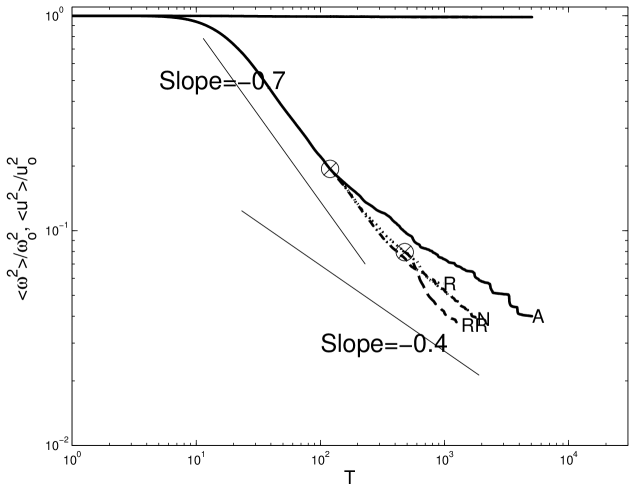
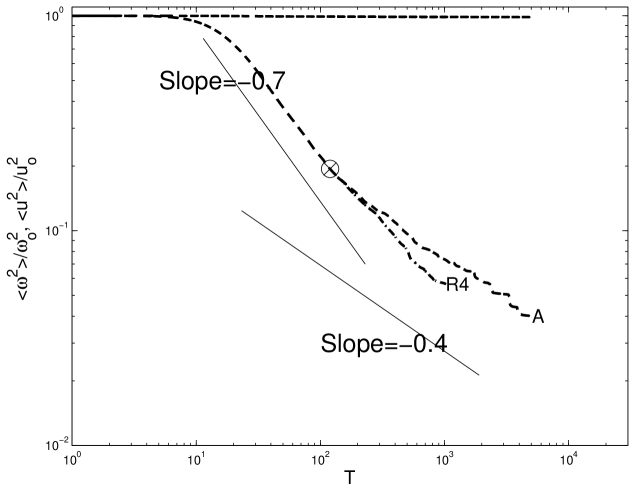
On Fig. 1 the time evolution of normalized enstrophy $\Omega(t)/\Omega(t=0)$ is presented. The curve A is the one obtained from the $512^{3}$ simulations reported in Ref.[7]. The cross-over from from the short-time magnitude of the decay exponent $\gamma\approx 0.7$ to the long -time asymptotics $\gamma\approx 0.4$ happening at the dimensionless time $T=t\omega_{0}\approx 120$ is clearly seen (curve A). To investigate the role of the large-scale modes in this phenomenon we, at the transition time $T\approx 120$ , randomized the phases of the first few modes ( $k\leq 5$ ) (curve R) and let the flow evolve. It is important to stress that this procedure influenced neither total enstrophy nor energy in the system. Still, the observed response of the flow to this perturbation was quite dramatic:

the randomization of phases of the modes, containing only a few percent of the total enstrophy, prevented transition from happening. Then, following the discussion with J.McWilliams, instead of randomizing, we at the same instant $T=120$ inverted the signs of the same modes in the unperturbed run $A$ , i.e. made a transformation $v_{i}(k)\rightarrow-v_{i}(k)$ with $k\leq 5$ . The effect of this procedure on the enstrophy evolution can be seen on Fig. 1a (curve N): the curves $R$ and $N$ are almost indistinguishable. After some time ( $T\approx 470$ ) the perturbed flow ( $R$ ) developed the large-scale coherent motions and a tendency to crossover to the long-time asymptotics ( $\gamma\approx 0.4$ ) could be detected. At this instant , again, the phases of the modes with $k\leq 5$ have been randomized. The result of this perturbation is shown on the curve $RR$ of Fig. 1a. We can see that the second randomization too, forced the enstrophy to decay much faster than $\Omega\propto t^{-0.4}$ observed in the dynamically unperturbed run $A$ . At this point we can make a definitive statement: the phase correlation , dynamically established as a result of the large-scale evolution, is crucial for the very existence of transition to the long-time enstrophy decay regime.

If the previous experiment established strong coupling between large ( $k\leq 5$ ) and small ( enstrophy containing) scales , then the next natural question to ask is: what is the minimal length-scale of the energy-containig structures influencing such small-scale phenomenon as the enstrophy decay process? To answer this question, we broadened our search. The phase randomization of the modes $v(k)$ with $k\leq 2$ did not show any effect on the decay process. The result of randomizing the phases of the modes with $k\leq 4$ containing at $T\approx 120$ less than five percent of total enstrophy $\Omega$ , is shown on Fig. 1b: the transition to the long -time behavior is delayed.

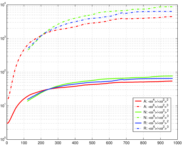
The time-dependence of the fourth and sixth-order moments are shown on Fig. 2. As we see, the initially gaussian random flow ( $t=0$ ) develops strongly non-gaussian tails characteristic of the small-scale vortex formation also observed in Ref.[10]. It is interesting that at the long times, the normalized high-order moments of the unperturbed vorticity field ( $A$ ) approach a close to steady state. Thus, in in accord with Ref.[11], we can write an exact equation for probability density $P(X)\equiv P(\frac{\omega}{\omega_{rms}})$ in terms of conditional expectation value of vorticity dissipation rate $Q(X)$ for a given magnitude of $X$ . A simple model $Q(X)\propto(1+kX^{2})$ proposed and numerically verified in Refs. [11] gives:

P(X)=\frac{C}{(1+\kappa X^{2})^{1+\frac{1}{2\kappa}}}

(1)

where $C$ is a normalization constant. After the transition ( $T>120$ ), the maximum value of vorticity in the evolving unperturbed field $\omega_{max}/\omega_{0}\approx 60\approx const$ and the expression (1) is valid in the interval $X_{max}\leq\omega_{max}/\omega_{rms}(t)$ . For $X>X_{max}$ , the probability density is cut off, i.e. we can set $P(X)\approx 0$ . It is due to the cut-off $X_{max}$ , the probability density (1) is consistent with the finite moments of vorticity field. Since $\omega_{rms}=O(t^{-0.2})$ , the magnitude of $X_{max}\propto t^{0.2}$ does not appreciably varies during the time of our simulation and can be set $X_{max}\approx const$ . The data (curves $A$ ) reported on Fig. 2 are reasonably well fitted by $\kappa\approx 1$ and $X_{max}\approx 30$ . As $\kappa\rightarrow 0$ , the relation (1) approaches a Gaussian and, since the evolution of the normalized moments is slow, the curves $A$ of Fig.2 can be represented by (1) with the time-dependent parameter $\kappa(t)$ . As we see from Fig.2, during the time of simulation, the sixth-order moments of perturbed runs $R$ and $N$ do not reach steady state meaning that the strong vortices decay with the exponent $\gamma_{s}<0.7$ .

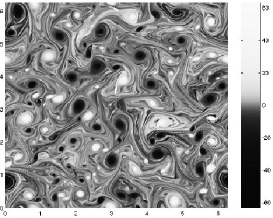
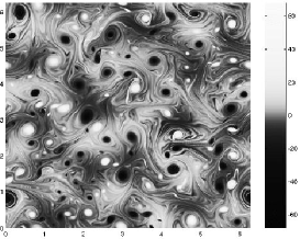
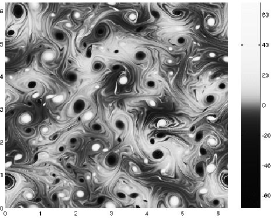
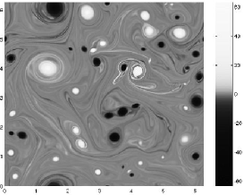
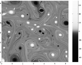
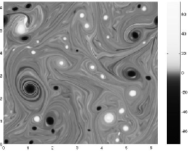
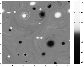
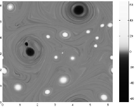
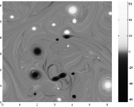
To make the discussion easier we will be dealing with three fields: 1. unperturbed (A); 2. randomized (R); and 3. sign-reversed (N). The time-evolution of vorticity field in all three runs (A; R N) is shown on Figs. 3-5. On Figs.3(A;R;N;) the vorticity fields at the transition time $T\approx 120$ right after randomization (Fig.3R) and sign reversal (Fig. 3N) are compared with the original unperturbed field (Fig. 3A). In all three plates we can identify the small-scale strong vortices which have not been affected by the randomization or sign-reversal. The patterns between these structures are quite different, though. The time-evolution of these fields presented on Figs.4-5 for the times $T\approx 480$ and $T\approx 975$ , respectively, leads to substantially different patterns: the larger number of strong vortices (also see below) can be seen in the field $A$ , while the evolution of the fields $R$ and $N$ results in the smaller number of vorticies. While during this evolution, the maximum value of vorticity stayed more or less unchanged ( $\omega_{max}\approx 65-60$ ), the number of strongest vortices having the peak value of vorticity $\omega_{o}\approx 0.8\omega_{max}$ (not shown here due to lack of space) in the unperturbed field $A$ was much larger (factor 1.5-4, depending on time $T$ ) than that in the corresponding perturbed runs $R$ and $N$ .

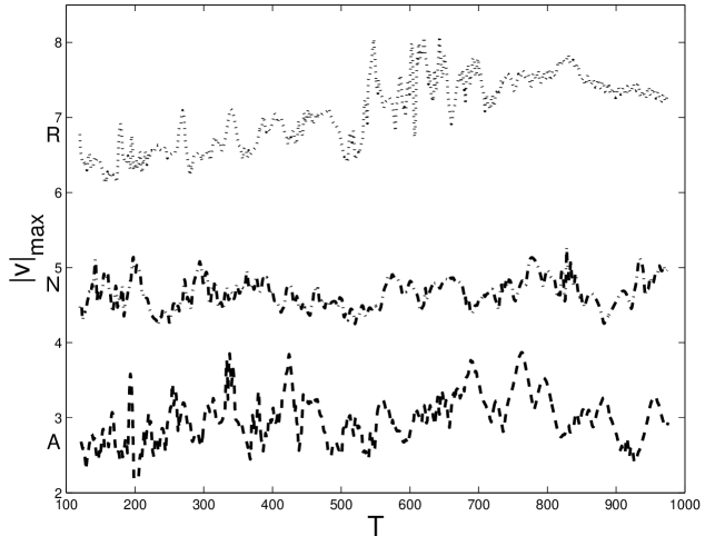
In Fig. 6 we show the time-evolution of maximum velocity $v_{max}$ in all three cases as a function of time. We can see that after some transient, the velocity in the unperturbed field $A$ reaches the values $v_{max}\approx 3.5-4.$ , while in the time interval $120<T<500$ the velocity in perturbed fields $R$ and $N$ is smaller: $v_{max}\approx 2.7-3.$ . It is interesting that by the time $T\approx 600$ , the maximum velocity of the field $R$ is more or less recovered while that in a stronger perturbed field $N$ remained substantially smaller than that in the $A$ -field during the remaining time of the simulation.

The strong correlation between small and large-scale structures in the small-scale forced 2D turbulence was discovered in Refs. [12]-[14]. Two different flow regimes were identified: at the short times, when the time-dependent integral scale $l_{I}\ll L$ , the inverse cascade led to generation of two -dimensional turbulence characterized by the Kolmogorov spectrum and close to gaussian magnitudes of the even-order moments velocity differences. The most interesting effect happened at the later times when the modes with $k\approx 1/L$ became populated: very strong vortices, were simultaneously formed at the forcing scale $l_{f}\approx 1/k_{f}$ . It was demonstrated¹³ that in the case of forced turbulence, the vortices were created at the centers of the large-scale, slowly -varying patterns where velocity $v\approx 0$ . Thus, the Bose condensate served as an almost steady well-organized matrix facilitating the vortex merger process. The possible generality of this phenomenon was demonstrated by the experiments of Paret and Tabeling¹⁴ in their investigation of time-evolution of the two-dimensional flow of mercury generated by magnetic field.

It is important to stress that, unlike in the forced flow considered in Refs. [12]-[14] where vorticity $\omega_{max}$ of the strongest vortices continuously grew with time, in decaying turbulence studied here, $\omega_{max}(t)\approx const\approx 60$ . If this feature persists for a very long time, eventually only two strong vorticis of the radius $a_{\infty}\approx[K/(\rho\omega_{max}^{2})]^{\frac{1}{4}}$ will be left in agreement with Ref.[1]. For the flow considered in this paper $a_{\infty}\approx 0.1$ . Thus, the final vortex occupies a tiny fraction ( $\approx 10^{-3}-10^{-4}$ ) of the flow. The flow velocity in this configuration will reach $v\approx a_{\infty}\omega_{max}\approx\sqrt{\omega_{max}}[K/\rho]^{\frac{1}{4}}\approx 5-10$ which is much larger than that in the initial random state. Thus, the 2D turbulence decay leads to formation of localized high-energy structures out of the initially quiescent background.

To conclude: the main result of the present study is: we have showed that the cross-over between the two asymptotics of enstrophy decay in 2D turbulence strongly depends upon fine details of the large-scale flow features containing very small fraction of total enstrophy $\Omega$ . The dynamic cause of this transition is not yet clear. However, we can conclude that fine, dynamically evolved, phase-correlation of the large-scale modes leads to a slower enstrophy decay and formation of more energetic flow structures. This points to a strong coupling between the small-scale and large-scale (condensates) structures in 2D turbulence. At the present time, we do not have a theory leading to this coupling and do not fully appreciate it’s consequences. Based on previous examples of coherent-random states interaction (superfluidity, superconductivity and many others) , the theory of the effect observed in this paper may be a substantial theoretical challenge. The possibility of this coupling in forced 2D turbulence was discussed by Polyakov¹⁵ in his conformal theory of two-dimensional turbulence. Since the geometry-dependent large-scale patterns cannot be universal, the question of universality of the transition is extremely interesting. The possible role of the inter-scale interaction, observed in this work, may be of great interest for meteorological applications.

We are grateful to J. McWilliams and A.Polyakov for valuable comments and suggestions.

References.
1. L. Onsager, Nuovo Cimento 6(2),279 (1949).
2 . J.C. McWilliams, J.Fluid Mech 219, 361 (1990).
3. G.F.Carnevale, J.C.McWilliams, Y.Pomeau, J.B.Weiss and W.R.Young, Phys.Rev.Lett.66, 2735 (1991).
4.A.Bracco, J.C.McWilliams, G.Murante,A.Provenzale,J.B.Weiss, Phys.Fluids 12, 2931 (2000).
5. M.V.Melander, J.C.McWilliams, and N.Zabusky, J.Fluid mech. 178, 137 (1987).
6. R.Benzi, S.Patarnello and P.Santangelo, J.Phys.A 21, 1221 (1988).
7. V.Yakhot and J.Wanderer, Phys.Rev.Lett.,93, 154502 (2004).
8. V.Yakhot, Phys.Rev.Lett., 93, 014502, 2004.
9. J.R.Chasnov, Phys. Fluids 9, 171 (1997).
10. L.M. Smith V. Yakhot, Phys.Rev.E55, 5458 (1997).
11. Ya.G. Sinai V.Yakhot, Phys.Rev.Lett., 63, 1962 (1989); V.Yakhot, S.Orszag, S. Balachandar, E. Jackson, Z.S.She, L.Sirovich, J.Sci.Comp.,7, 199 (1990).
12. L.M. Smith and V.Yakhot, Phys.Rev.Lett. 71, 352 (1993).
13. L.M. Smith and V. Yakhot, J.Fluid Mech. 274 (1994).
14 J. Paret and P. Tabeling, Phys. Fluids 12, 3126 (1998).
15. A. Polyakov, Nucl.Phys. 386, 367 (1993).

Large-Scale Coherence and Law of Decay of Two-Dimensional Turbulence

Abstract