A topological approach to neural complexity

Abstract

Considerable efforts in modern statistical physics is devoted to the study of networked systems. One of the most important example of them is the brain, which creates and continuously develops complex networks of correlated dynamics. An important quantity which captures fundamental aspects of brain network organization is the neural complexity $C(\mathbf{X})$ introduced by Tononi et al.. This work addresses the dependence of this measure on the topological features of a network in the case of gaussian stationary process. Both analytical and numerical results show that the degree of complexity has a clear and simple meaning from a topological point of view. Moreover the analytical result offers a straightforward and faster algorithm to compute the complexity of a graph than the standard one.

I. INTRODUCTION

The study of networked systems such as the Internet, social networks and biological networks has recently attracted great interest within the statistical physics community. A large variety of techniques and models have been developed in order to understand or predict the behavior of these systems. Great efforts have been applied in discovering their topological features ref1 ; ref2 ; ref3 ; ref4 and how these properties influence the behaviour of dynamical processes taking place on them. For example, we would like to know how the topology of social networks influences the spread of information social1 ; social2 , how the search engines are affected by World Wide Web structure www1 ; www2 .
In this paper we focus on a first basic approach for studying the interplay between dynamics and topology of brain networks.This study has great interest from several points of view: the brain and its structural features can be seen as a prototype of a physical system capable of highly complex and adaptable patterns in connectivity, selectively improved through evolution; architectural organization of brain cortex is one of the key features of how brain system evolves, adapts itself to the experience, and to possible injuries.
Brain activity can indeed be modelled as a dynamical process acting on a network; each vertex of the structure represents an elementary component, such as brain areas, groups of neurons or individual cells. A measure, called complexity, has been introduced ton with the purpose to get a sensible measure of two important features of the brain activity: segregation and integration. The former is a measure of the relative statistical independence of small subsets; the latter is the measure of statistical deviation from independence of large subsets.
Complexity is based on the values of the Shannon entropy calculated over the dynamics of the different sized subgraphs of the whole network. It is sensitive both to the statistical properties of the dynamics and to the connectivity.
It has been shown ton0 , by means of genetic algorithms, that the graphs showing high values of complexity are characterized by being both segregated and integrated; the complexity is low when the system is either completely independent (segregated), or completely dependent (integrated). This general behaviour is valid over a wide range of dynamical processes ton0 ; ton1 ; ton2 ; ton3 .

Despite this evidence, analytical results about the dependence of complexity on the topology and the dynamics is still lacking.
In the following will be proposed a first approach to this problem when the dynamics is gaussian. The use of the gaussian dynamics get the statistical measure of complexity independent from the dynamics itself. It doesn’t pretend to represent any realistic brain structure or activity, but to offer a first basic step for understanding the relation existing between values of complexity and topological properties of brain structure. For this reason we used a simplified version of the model introduced by ton1 . This is a first step which could be furtherly developed for example for directed and weighted graphs.

II.DYNAMICS, ENTROPY AND COMPLEXITY

We consider a graph composed by $n$ vertices and $m$ links. It can be represented by its adjacency matrix $\hat{\textbf{A}}$, whose elements $a_{ij}$ we set to $1$ if there is a link between the vertices $i$ and $j$, and $0$ otherwise. Only non self connections are considered and $a_{ij}=a_{ji}$.
On the graph we model the activity as a stochastic process in the following way: each node $i$ at time $t$ can be in a particular state defined by the quantity $X_{i}(t)$. Given our graph with $n$ nodes, the states of the whole graph at time $t$ is given by the $n-dimensional$ vector $\textbf{X}(t)$.

The evolution of $\textbf{X}(t)$ is given by the following dynamics:

$$\mathbf{X}(t+1) = \hat{\mathbf{C}}\cdot\mathbf{X}(t)+\mathbf{R}(t)$$

$$\mathbf{X}(0) = \mathbf{R}(0)$$ (1)

where $\hat{\textbf{C}}=\hat{\textbf{A}}/n$ and $\mathbf{R}(t)$ is an $n-dimensional$ vector whose components $R_{i}(t)$ are random values. $R_{i}(t)$ is chosen to be a white gaussian noise, i.e. with the following properties :

$$\overline{R}_{i}(t) = 0$$

$$\overline{R_{i}(t)R_{j}(t^{\prime})} = \sigma\delta_{ij}\delta(t-t^{\prime})$$ (2)

Here the bar represents the average over the ensemble.
The normalization $n$ of the adjacency matrix assures that the process will reach a stationary state. The dynamics, described by eq.(A topological approach to neural complexity), is indeed a random walk which is damped if the matrix has eingeinvalues $|{\lambda}|<1$. In such a way the dynamics reaches a stationary state with a caracteristic time $\tau\approx 1/\lambda_{min}$, where $\lambda_{min}$ is the smallest eingenvalues of the matrix $\hat{\mathbf{C}}-\hat{\mathbf{I}}$.
It is worth noting that the equation (A topological approach to neural complexity) represents a simplified version of the dynamics introduced in ton1 . In that case it was considered a gaussian dynamics on directed and weighted graphs and with some limitations on the values of the variances of each unit (node).

Since $\textbf{X}(t)$ is a multidimensional gaussian process, its statistics is completely described through its second order moment:

$$\overline{\mathbf{X}(t+1)\mathbf{X}^{t}(t+1)}=\hat{\mathbf{C}}\overline{\mathbf{X}(t)\mathbf{X}^{t}(t)}\hat{\mathbf{C}}^{t}+\hat{\mathbf{I}}$$ (3)

$\overline{\mathbf{X}(t+1)\mathbf{X}^{t}(t+1)}$ is the $n\times n$ covariance matrix whose determinant will be referred in the following as $|cov(\mathbf{X})|$. The average value of $\textbf{X}(t)$ is always zero being a sum of zero mean values at each time step.
Since the process $\mathbf{X(t)}$ is gaussian, it is possible to show that the Shannon entropy $H(\mathbf{X})$ depends only on $|cov(\mathbf{X})|$ pap :

$$H(\mathbf{X})=0.5\cdot\ln[{(2\pi e)^{n}|cov(\mathbf{X})|}]$$ (4)

Let us consider all the possible subgraphs of rank $\it{k}$ (number of nodes) of the whole graph. Each of these subgraphs are indicated as $\mathbf{X}_{k}$.

The complexity has been defined as:

$$C(\mathbf{X})=\sum_{k}\left[\langle H(\mathbf{X}_{k})\rangle-\frac{k}{n}H(\mathbf{X})\right]$$ (5)

where the average $\langle...\rangle$ is taken over all the subgraphs of rank $k$. The sum ranges from the minimum possible rank of a subgraph, i.e. $2$ to $n-1$. The term in (5) for $k=1$ would be trivial since the covariance matrix of disconnected vertices is simply dependent only on the variance of $\mathbf{R}(t)$, i.e. $|\mathbf{COV(\mathbf{X}_{1})}|=\sigma^{n}$; the term for $k=n$ is instead always null. In the following, we will set for the sake of simplicity $\sigma=1$.

In what follows we will try to find a relation between the topology of the graph and its values of Entropy $H(\mathbf{X})$ and Complexity $C(\mathbf{X})$, having defined on it the multidimensional gaussian process (A topological approach to neural complexity).

Under stationary conditions, the generic element of $cov(\mathbf{X})$ in the eigenvectors base $\textbf{x}^{\prime}_{i}$ is:

$$\overline{x^{\prime}_{i}x^{\prime}_{l}}=\frac{\delta_{il}}{1-\-\frac{\lambda_{i}}{n}\frac{\lambda_{l}}{n}}$$ (6)

The set of value $\lambda_{i}$ represents the eigenvalue spectrum of the adjacency matrix $\hat{\textbf{A}}$:

$$\sum_{j}A_{ij}x^{\prime}_{j}=\sum_{j}\lambda_{j}x^{\prime}_{j}\delta_{ij}$$ (7)

Following (6) the determinant of the covariance matrix is:

$$|cov(X)|=\prod_{i}\frac{1}{1-\frac{\lambda_{i}^{2}}{n^{2}}}\\$$ (8)

This expression shows that the dynamics depends only on the properties of the adjacency matrix $\hat{\textbf{A}}$ through its eigenvalue spectrum. As a consequence the statistical properties of the stationary states can be analized without studying their time evolution but by looking at their eigenvalue spectrum. On the other hand the richness in information embedded in the eigenvalue spectrum makes the analysis not trivial at all spectra . The aim of the next paragraph is to show which topological properties embedded into the spectrum dominate the behaviour of the dynamical process.

III. CONNECTION WITH THE TOPOLOGY

Using the equation (8), $H(\mathbf{X})$ becomes:

$$H(\mathbf{X}) = 0.5\cdot\ln[(2\pi e)^{n}|cov(\mathbf{X})|]$$ (9)

$$= 0.5\cdot\sum_{i}\ln\left[(2\pi e)\frac{1}{1-\frac{\lambda_{i}^{2}}{n^{2}}}\right]$$

If $\lambda_{max}^{2}/n^{2}<<1$, we can consider the following series expansion:

$$\ln\left(1-\frac{\lambda_{i}^{2}}{n^{2}}\right) \simeq -\sum_{i}\frac{\lambda_{i}^{2}}{n^{2}}-\sum_{i}\frac{\lambda_{i}^{4}}{2n^{4}}+$$ (10)

$$+ O\left(\sum_{i}\frac{\lambda_{i}^{6}}{3n^{6}}\right)$$

and by substitution in (9), we get:

$$H(\mathbf{X}) \simeq \ln(2\pi e)^{\frac{n}{2}}+0.5\left(\sum_{i}\frac{\lambda_{i}^{2}}{n^{2}}+\sum_{i}\frac{\lambda_{i}^{4}}{2n^{4}}\right)+$$ (11)

$$+ O\left(\sum_{i}\frac{\lambda_{i}^{6}}{6n^{6}}\right)$$

Eq.(11) allows us to relate $H(\mathbf{X})$ to the number $D_{k}$; this is the number of $k-step$ directed paths of the underlying -undirected- graph, which return to their starting node after $k$ steps:

$$D_{k}=\sum_{i=1}^{n}(\lambda_{i})^{k}=\sum_{i_{1},i_{2},...,i_{k}}a_{i_{1},i_{2}}a_{i_{2},i_{3}}...a_{i_{k},i_{1}}$$ (12)

where $a_{i_{k},i_{k+1}}$ is the generic non zero element of the adiancency matrix $\hat{\mathbf{A}}$.

Using this result $H(\mathbf{X})$ becomes:

$$H(\mathbf{X}) \simeq \ln(2\pi e)^{\frac{n}{2}}+0.5\left(\frac{D_{2}}{n^{2}}+\frac{D_{4}}{2n^{4}}\right)+$$ (13)

$$+ O\left(\frac{D_{6}}{6n^{6}}\right)$$

$D_{2}$ is then the number of paths which starting from any node $i$ go to any other one $j$ and then come back to $i$. Remembering that an unconnected pair of nodes has $a_{ij}=0$, $D_{2}$ is obviously twice the number of links of the whole graph.

Thus the first two terms of $H(\mathbf{X})$ expansion depend only on the number of nodes and links, and not on the graph topology.

Consider now the value of complexity $C(\mathbf{X})$ up to the $D_{2}$ term in the entropy. We get

$$C(\mathbf{X}) = \sum_{k=2}^{n-1}\left[\langle H(\mathbf{X}_{k})\rangle-\frac{k}{n}H(\mathbf{X})\right]\simeq$$ (14)

$$\simeq 0.5\sum_{k=2}^{n-1}\left(\frac{\langle D_{2}(k)\rangle}{k^{2}}-\frac{k}{n}\frac{D_{2}}{n^{2}}\right)=$$

$$= \sum_{k=2}^{n-1}\left(\frac{\langle m(k)\rangle}{k^{2}}-\frac{m}{n^{2}}\frac{k}{n}\right)=$$

$$= \frac{m(n-2)}{n(n-1)}-\frac{m(n+1)(n-2)}{2n^{3}}+\frac{m}{n^{3}}\sum_{k=2}^{n-1}\frac{1}{k}=$$

$$= C^{ord2}(n,m)$$

since:

$$\langle m(k)\rangle=m\frac{k(k-1)}{n(n-1)}$$

So far, the value of $C(\mathbf{X})$ is not defined by the topology. In order to reveal something related to a particular link’s arrangement, we need to consider the further terms in the expansion. We can rewrite the complexity $C(\mathbf{X})$ in the following way to put in evidence the part dependent only on the number of links $m$ and nodes $n$ of the whole graph (and so independent from the topology), $C^{ord2}(n,m)$:

$$C(\mathbf{X}) = C^{ord2}(n,m)+$$ (15)

$$+ \frac{1}{4}\sum_{k=2}^{n-1}\left(\frac{\langle D_{4}(k)\rangle}{k^{4}}-\frac{k}{n}\frac{D_{4}}{n^{4}}\right)+R(\lambda)$$

$$R(\lambda)=O\left[\sum_{k=2}^{n-1}\left(\sum_{i}\frac{\langle\lambda_{i}(k)^{6}\rangle}{6k^{6}}\right)-\frac{k}{n}\frac{D_{6}}{6n^{6}}\right]$$ (16)

where we have explicitly written the term in $\lambda^{4}$.

In order to express the topological information contained in the eq.(15), let us consider that

$$\langle D_{4}(k)\rangle = \langle\sum_{i}\lambda_{i}(k)^{4}\rangle=$$ (17)

$$= \langle 4m(k)^{2}\rangle-\sum_{i\neq j}\langle\lambda_{i}(k)^{2}\lambda_{j}(k)^{2}\rangle$$

and

$$\sum_{i\neq j}\lambda_{i}^{2}(k)\lambda_{j}^{2}(k)=\sum_{i\neq j}\sum_{lq}a_{il}a_{li}a_{jq}a_{qj}-2D_{2}(k)$$ (18)

From eq.(17) we see that the $C(\mathbf{X})$, at this order of approximation, depends on the second order moment of the number of links $\langle m(k)^{2}\rangle$, calculated over all the subgraphs of rank $k$ (we remember that a subgraph of rank $k$ is a particular choice of $k$ nodes in the whole graph and $k\in[2,n-1]$). This is the first quantity dependent on the topology that we can easily evaluate on the graph in place of the original expression of complexity. In the next step we will show that the fourth order approximated value of complexity can be expressed through $\langle m(k)^{2}\rangle$ calculated over all the subgraphs of rank $k$, (i.e. $k\in[2,n-1]$) and the second order moment of the degree distribution $\langle\langle q^{2}\rangle\rangle$ of the whole graph. This will allow to distinguish the complexity of graphs with the same total number of nodes $n$ and total number of links $m$, through the evaluation of less time consuming measures than the complexity. Moreover this result will offer a deeper understanding of what the complexity measure means from the topological point of view.

The terms in the sum of eq.(18) can be explicitly expressed as:

$$\begin{array}[]{lcl}&&\sum_{i\neq j}\sum_{lq}a_{il}a_{li}a_{jq}a_{qj}=\\ &&\\ &=&\sum_{i\neq j;l=j,q=i}(a_{ij}a_{ji})^{2}+\sum_{i\neq j\neq l\neq q}a_{il}a_{li}a_{jq}a_{qj}+\\ &&\\ &+&3\sum_{i\neq j\neq l}a_{il}a_{li}a_{jl}a_{lj}+2\sum_{i\neq j\neq l}a_{il}a_{il}a_{jj}a_{jj}+\\ &&\\ &+&\sum_{i\neq j;l=i,q=j}a_{ii}a_{ii}a_{jj}a_{jj}+2\sum_{i\neq jl=q=j}a_{ij}a_{ji}a_{jj}a_{jj}\\ \end{array}$$ (19)

In the expression (19), only the first three terms are non zero, while the others contain at least a diagonal element $a_{ii}=0$. Moreover the first term is just $D_{2}$.

It is easy to show that the second and the third terms in the sum correspond to the number of paths (“loops”) of the type shown in Fig. 1:

Figure 1: top: paths described by the third term in eq.(19); bottom: paths described by the second term in eq.(19)

We will show that the number of these paths is related to $\langle\langle q^{2}\rangle\rangle$. In what follows $\it{q}$ represents the degree of the generic node $\it{i}$, i.e. the node $\it{i}$ has $\it{q}$ links.

Consider now a particular subgraph of rank k. It has k nodes, each of them having a certain number of links or none. Consider then all the nodes having the same degree $\it{q}$ in a generic subgraph of rank $\it{k}$; then the number of paths (loops) of the first type in Fig.1, involving this kind of nodes are:

$${n-3\choose k-3}\cdot{q\choose 2}$$

where ${n-3\choose k-3}$ is the number of ways to choose $\it{k}$ nodes over a total of $\it{n}$ nodes, leaving aside the 3 nodes which belong to the pair considered. This is the number of subgraph of rank k, in the whole graph, which contain a particular choice of 3 nodes. Moreover, since the generic node $\it{i}$ has $\it{q}$ links, we can count ${q\choose 2}$ different pairs of links sharing the same node $\it{i}$.
If we denote with $P(q)$ the degree distribution in the whole graph, then we can write the third term in eq.(19) as :

$$\sum_{\{k\}}\sum_{i\neq j\neq l}a_{il}a_{li}a_{jl}a_{lj} = \int_{1}^{q_{max}}{n-3\choose k-3}{q\choose 2}P(q)dq=$$

$$= \frac{1}{2}{n-3\choose k-3}(\langle\langle q^{2}\rangle\rangle-\langle\langle q\rangle\rangle)$$

where we explicitely wrote the $\sum_{\{k\}}$ which we will use later. $\sum_{\{k\}}$ means the sum over all the subgraphs with $\it{k}$ nodes or of rank k.
Consider now the second term in eq.(19), i.e. $\sum_{i\neq j\neq k\neq q}a_{ik}a_{ki}a_{jq}a_{qj}$. This is the number of disjoint pairs of links in a generic subgraph of rank $\it{k}$.
To compute such number, we first count the total number of pairs in the whole graph, i.e. ${m\choose 2}$; then we subtract the number of pairs of links sharing a node in the whole graph (from the previous computation). Finally we have to consider the multiplicity ${n-4\choose k-4}$, i.e. the number of subgraphs of rank $\it{k}$ containing each pair of disjoint links.
Then the second term in eq.(19) is (again considering also the sum: $\sum_{\{k\}}$) :

$$\sum_{\{k\}}\sum_{i\neq j\neq l\neq q}a_{il}a_{li}a_{jq}a_{qj} = \left[{m\choose 2}-\frac{1}{2}(\langle\langle q^{2}\rangle\rangle-\langle\langle q\rangle\rangle)\right]$$

$$\cdot {n-4\choose k-4}$$

Remembering that in eq.(15) we have to compute the quantity $\sum_{k=2}^{n-1}\langle D_{4}(k)\rangle$, then we have to evaluate $\sum_{k=2}^{n-1}\sum_{i\neq j}\sum_{lq}\langle a_{il}a_{li}a_{jq}a_{qj}\rangle$. The average $\langle...\rangle$ is performed for a particular value of k over all the subgraph of rank k. For this reason in previous expressions we have explicitely written the sum over all the subgraphs of rank k, i.e. $\sum_{\{k\}}$. To perform the average $\langle...\rangle$ we have then simply to divide such expressions for the number of subgraph of rank k contained in the whole graph, i.e.$n\choose k$. Eventually we have to sum over all the values of k, $\sum_{k}$.

Then the final expression for $\sum_{k}\langle D_{4}(k)\rangle$ becomes:

$$\begin{array}[]{lcl}\sum_{k}\langle D_{4}(k)\rangle=\sum_{k}\langle 4m(k)^{2}\rangle+\sum_{k=2}^{k=n-1}\frac{\langle 2m(k)\rangle}{{n\choose k}}\\ &\\ +\frac{1}{2}\sum_{k=4}^{n-1}(\langle\langle q^{2}\rangle\rangle-\langle\langle q\rangle\rangle)\frac{{n-4\choose k-4}}{{n\choose k}}-{m\choose 2}\sum_{k=4}^{n-1}\frac{{n-4\choose k-4}}{{n\choose k}}\\ &\\ +\frac{3}{2}\sum_{k=3}^{n-1}(\langle\langle q\rangle\rangle-\langle\langle q^{2}\rangle\rangle)\frac{{n-3\choose k-3}}{{n\choose k}}\end{array}$$ (20)

where the second and third term of eq.(19) have been substituted with their explicit computations.
It is worth to note that $\sum_{k=2}^{n-1}\langle\langle q\rangle\rangle$ is only a function of $\it{n}$ and $\it{m}$, being $\langle\langle q\rangle\rangle=\frac{m}{n}$.

In the following is the whole expression of $C(X)$:

$$\begin{array}[]{lcl}C(X)=C^{ord2}(n,m)+C^{ord4}_{1}(m,n,\sum_{k=2}^{n-1}\langle m(k)^{2}\rangle)+\\ &\\ +C^{ord4}_{2}(m,n,\langle\langle q^{2}\rangle\rangle)+C^{ord4}_{3}(m,n,\langle\langle q\rangle\rangle)+\\ &\\ +C^{ord4}_{4}(m,n)+R(\lambda)\end{array}$$ (21)

where $C^{ord2}(n,m)$ and $R(\lambda)$ are respectively the eq.(14) and eq.(16). The other terms are:

$$\begin{array}[]{lcl}C^{ord4}_{1}(m,n,\sum_{k=2}^{n-1}\langle m(k)^{2}\rangle)=\sum_{k=2}^{n-1}\frac{\langle m(k)^{2}\rangle}{k^{4}}\\ &\\ &\\ C^{ord4}_{2}(m,n,\langle\langle q^{2}\rangle\rangle)=\frac{\langle\langle q^{2}\rangle\rangle}{8}\frac{n^{2}-n-3}{n^{4}}+\\ &\\ +\frac{\langle\langle q^{2}\rangle\rangle}{8}\left(\sum_{k=4}^{n-1}\frac{1}{k^{4}}\frac{(n-4)!k!}{(k-4)!n!}-\sum_{k=3}^{n-1}\frac{3}{k^{4}}\frac{(n-3)!k!}{(k-3)!n!}\right)\\ &\\ &\\ C^{ord4}_{3}(m,n,\langle\langle q\rangle\rangle)=-\frac{1}{8}\frac{n^{2}-n-3}{n^{4}}+\\ &\\ +\frac{1}{8}\left(\sum_{k=3}^{n-1}\frac{3}{k^{4}}\frac{(n-3)!k!}{(k-3)!n!}-\sum_{k=4}^{n-1}\frac{1}{k^{4}}\frac{(n-4)!k!}{(k-4)!n!}\right)\\ &\\ &\\ C^{ord4}_{4}(m,n)=-\frac{m(n+1)(n-2)}{4n^{5}}+\\ &\\ +\frac{m}{2}\left(\sum_{k=2}^{k=n-1}\frac{1}{n(n-1)}\frac{1}{{n\choose k}}\frac{k-1}{k^{3}}-\frac{m-1}{4}\frac{{n-4\choose k-4}}{{n\choose k}}\frac{1}{k^{4}}\right)\\ \end{array}$$

Figure 2: 3 different network models: a regular network, the small word model and a random network. It is possible to go from one model to the other varying the probability $p$ of rewiring (see the text for further details).

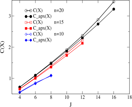
Figure 3: Behaviour of complexity measure and its approximation (up to the fourth order) in a small world graph with n=10,15,20 nodes and p=0.1, against J, i.e. number of first neighbors.

[htbp]

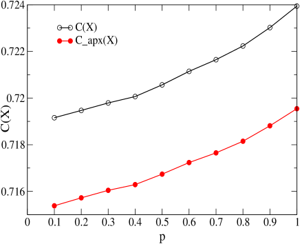
Figure 4: Behaviour of complexity measure and its approximation (up to the fourth order) in a small world graph with n=20 nodes and J=4, against p, probability of rewiring.

IV. NUMERICAL RESULTS

We perform calculation of entropy and complexity of the dynamics (A topological approach to neural complexity) over a small world graph with $n=10,15,20$ nodes. We estimate both the exact and the approximate values, for checking the accuracy of the approximation, and their dependence on the topological properties of the graphs.

The algorithm behind the model can be summarized in two steps wat :
(1) Start with a ring lattice with $\it{n}$ nodes in which every node is connected to its first $\it{J}$ neighbors ($\it{J/2}$ on either side). In order to have a sparse but connected network at all times, consider $n>>J>>ln(n)>>1$.
(2) Randomly rewire each edge of the lattice with probability $\it{p}$ such that self-connections and duplicate edges are excluded. Varying $\it{p}$ the transiton between order $(p=0)$ and randomness $(p=1)$ can be closely monitored (Fig.2).

The numerical evaluation for the exact and the approximated values of $C(\mathbf{X})$ can be easily achieved in a small world graph: in this case we can investigate different arrangements of links keeping the number of nodes and links fixed. The variation of complexity is affected both by $\langle m(k)^{2}\rangle$ over all the scales $\it{k}$, and $\langle\langle q^{2}\rangle\rangle$.

Since the expansion is allowed when the average node degree is much less than one ($\lambda_{max}^{2}/n^{2}<<1$), we expect a higher accuracy when the average connectivity is low ($n>>J$), and a worse approximation when $\it{J}$ increases. The simulations confirm this trend for increasing values of $\it{J}$, and $J<n$ (Fig. 3).
In Fig.4 we show the exact and approximated behaviour of $C(\mathbf{X})$ versus the probability of rewiring.Their relative difference is much less than one and they show very similar behaviour.
Analogous results have been found for the other values of $\it{n}$.

V. DISCUSSION

We attempted to extract the topological meaning of the complexity measure in the case of gaussian dynamic. This aim has been achieved both from analytical and numerical points of view, showing that very good approximation of complexity can be obtained through two simple direct topological measures on the graph, namely, the second order moment of the number of links $\langle m^{2}(k)\rangle$ over all the scales $\it{k}$, and the second order moment of the node degree $\langle\langle q^{2}\rangle\rangle$ on the whole graph. The analytical expression is obtained through an expansion for $\lambda_{max}/n<<1$; however the numerical results show the expression (21) for the complexity is a reasonable approximation even for $\lambda_{max}/n\lessapprox 1$.
The relevance of the obtained results relies on two main aspects: the measure has a clear topological meaning which help to understand in a more intutive way the degree of complexity of a graph; it can be evaluated through two less time-consuming, and considerably easier to compute topological measures. The saving of computation time is of order $\it{n}$ since evaluating the two mesures mentioned above require $\it{n^{2}}$ steps instead of the $\it{n^{3}}$ steps of the diagonalizing algorithms for symmetric matrices.

We enjoyed useful discussions and suggestions by Dr.V.Servedio and Dr.A. Capocci. We would like to thank Dr. F.Colaiori for her help in drawing figures.

References

• (1) S. H. Strogatz, Nature 410, 268-276 (2001)
• (2) R. Albert and A.-L. Barabási, Rev. Mod. Phys. 74, 47-97 (2002), and references therein
• (3) A.-L. Barabási and R. Albert, Science 286, 509-512 (1999).
• (4) S.N.Dorogovtsev and J.F.F. Mendes, Adv. Phys. 51, 1079-1187 (2002).
• (5) M. E. J. Newman, Proc. Nat. Acad. Sci. USA 98, 404-409 (2001.)
• (6) A.-L. Barabási, H. Jeong, E. Ravasz, Z. Néda, A. Shubert and T. Vicsek, Physica A 311, 590-614 (2002).
• (7) R. Cohen, K. Erez, D. ben-Avraham and S. Havlin, Phys Rev Lett 85, 4626-4628 (2000).
• (8) A.-L. Barabási, R. Albert, Jeong H., and Bianconi G., Science 287, 2115a (2000).
• (9) G. Tononi, O. Sporns, and G.M. Edelman, Proc. Nat. Acad. Sci. USA 91, 5033-5037 (1994.)
• (10) O. Sporns and G. Tononi, Complexity 7 (1), 28-38 (2002).
• (11) O. Sporns, G. Tononi, and G.M. Edelman, Cereb. Cortex 10(2), 127-141 (2000).
• (12) O. Sporns, G. Tononi, and G.M. Edelman, Neural Networks 13 (8-9), 909-922 (2000).
• (13) O. Sporns, G. Tononi, G. M. Edelman, Behavioural Brain Research 135 (1-2), 69-74 (2002)
• (14) A. Papoulis, Probability, Random variables, Stochastic processes (McGraw-Hill, New York, (1991)).
• (15) I. J. Farkas, I. Derenyi, and A.-L. Barabási, T. Vicsek, Phys. Rev. E 64, 026704-026715 (2001).
• (16) D. J. Watts, and S. H. Strogatz, Nature 393, 440-442 (1998).