Models for optical solitons in the two-cycle regime

H. Leblond and F. Sanchez

Laboratoire POMA, UMR 6136, Université d’Angers, 2 Bd Lavoisier, 49000 Angers, France

Abstract

We derive model equations for optical pulse propagation in a medium described by a two-level Hamiltonian, without the use of the slowly varying envelope approximation. Assuming that the resonance frequency of the two-level atoms is either well above or well below the inverse of the characteristic duration of the pulse, we reduce the propagation problem to a modified Korteweg-de Vries or a sine-Gordon equation. We exhibit analytical solutions of these equations which are rather close in shape and spectrum to pulses in the two-cycle regime produced experimentally, which shows that soliton-type propagation of the latter can be envisaged.

1 Introduction

Recent advances in dispersion managing now allow the generation of ultrashort optical pulses containing few oscillations directly from a laser source. Two-cycle pulses have been recently reported in mode-locked Ti-sapphire lasers using double-chirped mirrors [1, 2, 3]. Because the pulse duration becomes close to the optical period, a question of interest is to know if few cycle pulses can generate optical solitons in nonlinear media. The usual description of short pulses propagation in nonlinear optics is made using the nonlinear Schrödinger (NLS) equation which is derived using the slowly varying envelope approximation. However, for ultrashort pulses considered in this paper the slowly varying envelope approximation is not valid any more. This situation, and the corresponding one in the spatial domain, called ‘non-paraxial’, have already given rise to several studies. An approach consists in adding corrective terms to the NLS model [4]. This high-order perturbation approach still involves the slowly varying envelope approximation, and requires cumbersome and difficult computations. The approach of [5] allows one to determine the ray trajectories in a very rigorous way, without any use of the paraxial approximation. However, it still makes use of the slowly varying envelope approximation in the time domain, and therefore can hardly be generalized to the problem under consideration in this paper. It is preferable to leave completely the concept of envelope. Indeed, it is not adapted when a pulse is composed of few optical cycles. The aim of this paper is to demonstrate that other approximations can be envisaged and can also lead to completely integrable equations, and support solitons. The basic principle of our work is that a soliton can propagate only when the absorption is weak, therefore its characteristic frequency must be far away from the absorption range of the material. If it is far below, a long-wave approximation can be performed. On the other hand, if it is far above, it will be a short-wave approximation. Both approaches are used in this paper leading to completely integrable systems. It is organized as follows. In section 2 we develop the model which is based on a non absorbing homogeneous and isotropic two-level medium. A semi-classical approach is used leading to the well-known Maxwell-Bloch equations. The long-wave approximation is investigated in section 3. In this case the model reduces to a modified Korteweg-de Vries (mKdV) equation. The two-soliton solution is very close to the experimentally observed two-cycle pulses. In section 4 we investigate the short-wave approximation. The resulting model is formally equivalent to that describing the self-induced transparency. It can be reduced to the sine-Gordon equation. Again, the two-soliton solution is comparable with the experimental observations [3].

2 Model

In this section we derive the starting equations for further analysis. The medium is treated using the density matrix formalism and the field using the Maxwell equations.

We consider an homogeneous medium, in which the dynamics of each atom is described by a two-level Hamiltonian

$$H_{0}=\hbar\left(\begin{array}[]{cc}\omega_{a}&0\\ 0&\omega_{b}\end{array}\right).$$ (1)

A more realistic description should take into account an arbitrary number of atomic levels. Indeed, we consider wave frequencies far from the resonance line of the medium, and in this situation all transitions should be taken into account. But we intend here to suggest a new approach to the description of ultrashort optical pulses. Therefore we restrict the study to a very simple and rather academic model.

The atomic dipolar electric momentum is assumed to be along the $x$-axis. It is thus described by the operator $\vec{\mu}=\mu\vec{e}_{x}$, where $\vec{e}_{x}$ is the unitary vector along the $x$-axis and

$$\mu=\left(\begin{array}[]{cc}0&\mu\\ \mu^{\ast}&0\end{array}\right).$$ (2)

The polarization density $\vec{P}$ is related to the density matrix $\rho$ through

$$\vec{P}=N\mbox{tr}(\rho\vec{\mu}),$$ (3)

where $N$ is the number of atoms per unit volume. Thus $\vec{P}$ reduces to $P\vec{e}_{x}$.

The electric field $\vec{E}$ is governed by the Maxwell equations. In the absence of magnetic effects, and assuming that the wave is a plane wave propagating along the $z$-axis, polarized along the $x$-axis, $\vec{E}=E\vec{e}_{x}$, they reduce to

$$\partial_{z}^{2}E=\frac{1}{c^{2}}\partial_{t}^{2}(E+4\pi P).$$ (4)

$c$ is the light velocity in vacuum. We denote by $\partial_{t}$ the derivative operator $\frac{\partial}{\partial t}$ with regard to the time variable $t$, and so on.

The coupling between the atoms and the electric field is taken into account by a coupling energy term in the total Hamiltonian $H$, that reads:

$$H=H_{0}-\mu E.$$ (5)

The density matrix evolution equation (Schrödinger equation) writes as

$$i\hbar\partial_{t}\rho=\left[H,\rho\right]+{\cal R},$$ (6)

where $\cal R$ is some phenomenological relaxation term. The set of equations (4-6) is sometimes called the Maxwell-Bloch equations, although this name denotes more often a reduction of it.

Setting

$$t^{\prime}=ct\quad,\quad P^{\prime}=4\pi P\quad,\quad\rho^{\prime}=4\pi N\hbar c\rho\quad,\quad\mu^{\prime}=\frac{\mu}{\hbar c},$$ (7)

$$H^{\prime}=\frac{H}{\hbar c}\quad,\quad H_{0}^{\prime}=\frac{H_{0}}{\hbar c}\quad,\quad\omega_{a,b}^{\prime}=\frac{\omega_{a,b}}{c},$$ (8)

allows one to replace the constants $c$, $N$, $\hbar$ and $4\pi$ in system (3-6) by 1. We denote the components of $\rho$ by

$$\rho=\left(\begin{array}[]{cc}\rho_{a}&\rho_{t}\\ \rho_{t}^{*}&\rho_{b}\end{array}\right),$$ (9)

and so on, and by $\Omega=\omega_{b}-\omega_{a}$ the resonance frequency of the atom.

The relaxation expresses as

$${\cal R}=i\hbar\left(\begin{array}[]{cc}\rho_{b}/\tau_{b}&-\rho_{t}/\tau_{t}\\ -\rho_{t}^{*}/\tau_{t}&-\rho_{b}/\tau_{b}\end{array}\right),$$ (10)

where $\tau_{b}$ and $\tau_{t}$ are the relaxation times for the populations and for the coherences respectively. We show below that, according to the fact that relaxation occurs very slowly with regard to optical oscillations, the relaxation term $\cal R$ could be omitted.

3 Long-wave approximation

3.1 A modified Korteweg-de Vries equation

Let us first consider the situation where the wave duration $t_{w}$ is long with regard to the period $t_{r}=2\pi/\Omega$ (recall that $\Omega=\omega_{b}-\omega_{a}$) that corresponds to the resonance frequency of the two-level atoms. We assume that $t_{w}$ is about one optical period, say about one femtosecond. Thus we assume that the resonance frequency $\Omega$ is large with regard to optical frequencies. In order to obtain soliton-type propagation, nonlinearity must balance dispersion, thus the two effects must arise simultaneously in the propagation. This involves a small amplitude approximation. Further, we can speak of soliton only if the pulse shape is kept on a large propagation distance. Therefore we use the reductive perturbation method as defined in [6]. We expand the electric field $E$, the polarization density $P$ and the density matrix $\rho$ as power series of a small parameter $\varepsilon$ as

$$E=\sum_{n\geqslant 1}\varepsilon^{n}E_{n}\quad,\quad P=\sum_{n\geqslant 1}\varepsilon^{n}P_{n}\quad,\quad\rho=\sum_{n\geqslant 0}\varepsilon^{n}\rho_{n},$$ (11)

and introduce the slow variables

$$\tau=\varepsilon\left(t-\frac{z}{V}\right)\quad,\quad\zeta=\varepsilon^{3}z.$$ (12)

Expansion (11) gives an account of the small amplitude approximation. The retarded time variable $\tau$ describes the pulse shape, propagating at speed $V$ in a first approximation. Its order of magnitude $\varepsilon$ gives account for the long-wave approximation, so that the pulse duration $t_{w}$ has the same order of magnitude as $t_{r}/\varepsilon$. The propagation distance is assumed to be very long with regard to the pulse length $ct_{w}$, therefore it will have the same order of magnitude as $ct_{r}/\varepsilon^{n}$, where $n\geqslant 2$. The value of $n$ is determined by the distance at which dispersion effects occur. According to the general theory of the derivation of KdV-type equations [6], it is $n=3$. The $\zeta$ variable of order $\varepsilon^{3}$ describes thus long-distance propagation. The physical values of the relaxation times $\tau_{b}$ and $\tau_{t}$ are in the picosecond range, or even slower, thus very large with regard to the pulse duration $t_{w}$. Therefore we write

$$\tau_{j}=\frac{\hat{\tau}_{j}}{\varepsilon^{2}}\quad\mbox{ for $j=b$ and~{}$t$.}$$ (13)

The Schrödinger equation (6) at order $\varepsilon^{0}$ is satisfied by the following value of $\rho_{0}$, which represents a steady state in which all atoms are in their fundamental state $a$:

$$\rho_{0}=\left(\begin{array}[]{cc}\alpha&0\\ 0&0\end{array}\right).$$ (14)

Notice that, according to the change of variables (7), the trace $\mbox{tr}(\rho)$ of the density matrix is not 1 but $\alpha=4\pi N\hbar c$. Then the Schrödinger equation (6) at order $\varepsilon^{1}$ yields

$$\rho_{1t}=\frac{\mu\alpha}{\Omega}E_{1},$$ (15)

so that

$$P_{1}=\frac{2|\mu|^{2}\alpha}{\Omega}E_{1}.$$ (16)

The Maxwell equation (4) at order $\varepsilon^{3}$ gives the value of the velocity

$$V=\left(1+\frac{2|\mu|^{2}\alpha}{\Omega}\right)^{\frac{-1}{2}},$$ (17)

in accordance with the limit of the dispersion relation as the frequency $\omega$ tends to zero.

The Schrödinger equation (6) at order $\varepsilon^{2}$ yields $\rho_{1a}=\rho_{1b}=0$ and

$$\rho_{2t}=\frac{\mu\alpha}{\Omega}E_{2}-\frac{i\mu\alpha}{\Omega^{2}}\partial_{\tau}E_{1}.$$ (18)

Then

$$P_{2}=\frac{2|\mu|^{2}\alpha}{\Omega}E_{2},$$ (19)

and the Maxwell equation (4) at order $\varepsilon^{4}$ is automatically satisfied.

The Schrödinger equation (6) at order $\varepsilon^{3}$ gives

$$\rho_{2b}=-\rho_{2a}=\frac{|\mu|^{2}\alpha}{\Omega^{2}}E_{1}^{2}$$ (20)

and

$$\rho_{3t}=\frac{\mu\alpha}{\Omega}E_{3}-\frac{i\mu\alpha}{\Omega^{2}}\partial_{\tau}E_{2}-\frac{\mu\alpha}{\Omega^{3}}\partial_{\tau}^{2}E_{1}-\frac{2\mu|\mu|^{2}\alpha}{\Omega^{3}}E_{1}^{3}-\frac{i\mu\alpha}{\Omega^{2}\tau_{t}}E_{1}.$$ (21)

The corresponding term of the polarization density $P$ contains a nonlinear term:

$$P_{3}=\frac{2|\mu|^{2}\alpha}{\Omega}E_{3}-\frac{2|\mu|^{2}\alpha}{\Omega^{2}}\partial_{\tau}^{2}E_{1}-\frac{4|\mu|^{4}\alpha}{\Omega^{3}}E_{1}^{3},$$ (22)

but the terms involving the relaxation do not appear. The Maxwell equation at order $\varepsilon^{5}$ yields the following evolution equation for the main electric field amplitude $E_{1}$:

$$\partial_{\zeta}E_{1}=\frac{V|\mu|^{2}\alpha}{\Omega^{3}}\partial_{\tau}^{3}E_{1}+\frac{2V|\mu|^{4}\alpha}{\Omega^{3}}\partial_{\tau}E_{1}^{3},$$ (23)

which is a mKdV equation. Equation (23) can be generalized as follows: a general derivation of KdV-type models [7] shows that the coefficient of the dispersive term $\partial_{\tau}^{3}E_{1}$ in this equation must be $(1/6){d^{3}k}/{d\omega^{3}}$. We check by direct computation of the dispersion relation that it holds in the present case. Another heuristic reasoning can relate the value of the nonlinear coefficient of equation (23) to the third order nonlinear susceptibility $\chi^{(3)}$. It uses the nonlinear Schrödinger (NLS) equation which describes the evolution of a short pulse envelope in the same medium. The NLS equation writes as ([8], 6.5.32)

$$i\partial_{\zeta}{\cal E}-\frac{1}{2}k_{2}\partial_{\tau}^{2}{\cal E}+\gamma{\cal E}\left|{\cal E}\right|^{2}=0,$$ (24)

where $\cal E$ is the envelope amplitude of the wave electric field, $k_{2}$ the group velocity dispersion, and $\gamma$ is related to $\chi^{(3)}$ through

$$\gamma=\frac{6\omega\pi}{nc}\chi^{(3)}.$$ (25)

$n$ is the refractive index of the medium, $\omega$ the wave pulsation. We drop the dispersion term, replace $\omega$ by $i\partial_{\tau}$, and notice that $\cal E$ coincides with the real field $E_{1}$ at the long-wave limit, to get

$$\partial_{\zeta}E_{1}=\frac{-6\pi}{nc}\chi^{(3)}\partial_{\tau}E_{1}^{3}.$$ (26)

Equation (26) gives an expression of the nonlinear coefficient in the mKdV equation (23). The relevant component of the third order nonlinear susceptibility tensor $\chi^{(3)}$ computed from the above model is [8]

$$\chi^{(3)}_{xxxx}(\omega,\omega,\omega,-\omega)=-\frac{4}{3}\frac{N}{\hbar^{3}}\frac{\Omega|\mu|^{4}}{\left(\omega^{2}-\Omega^{2}\right)^{2}}\;.$$ (27)

Taking the long-wave limit $\omega\longrightarrow 0$ in equation (27), we check that the expression of the nonlinear coefficient obtained from (26) holds in the present case. Thus we can write equation (23) as

$$\partial_{\zeta}E_{1}=\frac{1}{6}\left.\frac{d^{3}k}{d\omega^{3}}\right|_{\omega=0}\partial_{\tau}^{3}E_{1}-\left.\frac{6\pi}{nc}\chi^{(3)}_{xxxx}(\omega,\omega,\omega,-\omega)\right|_{\omega=0}\partial_{\tau}E_{1}^{3}\;.$$ (28)

It can be reasonably conjectured that equation (28) will still hold in the more general case of an arbitrary number of atomic levels, when the inverse of the characteristic pulse duration is much smaller than any of the transition frequencies of the atoms.

3.2 The two-soliton solution

The mKdV equation (23) is completely integrable by means of the inverse scattering transform [9]. The $N$-soliton solution has been given by Hirota [10]. In order to write it easily, we write the mKdV equation (23) into the dimensionless form

$$\partial_{Z}u+2\partial_{T}u^{3}+\partial_{T}^{3}u=0,$$ (29)

where $u$ is a dimensionless electric field, and $Z$ and $T$ dimensionless space and time variables defined by

$$u=\frac{E_{1}}{E_{0}}\quad,\quad Z=\frac{-\zeta}{L}\quad\quad T=\frac{\tau}{T_{0}}.$$ (30)

The characteristic electric field, space and time are defined by

$$E_{0}=\frac{\Omega}{|\mu|}\quad,\quad T_{0}=\frac{1}{\Omega}\quad,\quad L=\frac{1}{\alpha|\mu|^{2}V},$$ (31)

in normalized units. Relations (30-31) can be expressed in a more convenient way as follows. Let us first choose as reference time the pulse length $t_{w}$ (in physical unit). The small perturbative parameter is then

$$\varepsilon=\frac{1}{t_{w}\Omega}.$$ (32)

The characteristic electric field $\cal E$, and propagation distance $\cal L$, are

$${\cal E}=\frac{\hbar}{t_{w}|\mu|}\quad,\quad{\cal L}=\frac{\hbar c^{2}\Omega^{3}t_{w}^{3}}{4\pi NV|\mu|^{2}},$$ (33)

where the speed $V$ is

$$V=c\left(1+\frac{8\pi|\mu|^{2}N}{\hbar\Omega}\right)^{\frac{-1}{2}}.$$ (34)

Then the quantities involved by the dimensionless equation (29) are related to the quantities measured in the laboratory through

$$u=\frac{E}{\cal E}\quad,\quad Z=\frac{-z}{\cal L}\quad,\quad T=\frac{1}{t_{w}}\left(t-\frac{z}{V}\right).$$ (35)

The soliton solution writes as

$$u=p\,\mbox{sech}\,\eta,$$ (36)

with

$$\eta=pT-p^{3}Z-\gamma,$$ (37)

$p$ and $\gamma$ being arbitrary parameters.

The two-soliton solution is

$$u=\frac{e^{\eta_{1}}+e^{\eta_{2}}+\left(\frac{p_{1}-p_{2}}{p_{1}+p_{2}}\right)^{2}\left(\frac{e^{\eta_{1}}}{4p_{1}^{2}}+\frac{e^{\eta_{2}}}{4p_{2}^{2}}\right)e^{\eta_{1}+\eta_{2}}}{1+\frac{e^{2\eta_{1}}}{4p_{1}^{2}}+\frac{2}{(p_{1}+p_{2})^{2}}e^{\eta_{1}+\eta_{2}}+\frac{e^{2\eta_{2}}}{4p_{2}^{2}}+\left(\frac{p_{1}-p_{2}}{p_{1}+p_{2}}\right)^{4}\frac{e^{2\eta_{1}+2\eta_{2}}}{16p_{1}^{2}p_{2}^{2}}}\;,$$ (38)

with

$$\eta_{j}=p_{j}T-p_{j}^{3}Z-\gamma_{j}\,,$$ (39)

for $j=1$ and 2. The parameters $p_{1}$, $p_{2}$, $\gamma_{1}$ and $\gamma_{2}$ are arbitrary. When they take real values, the explicit solution (38) describes the interaction of two localized bell-shaped pulses, which are solitons. An example of this solution is drawn on figure 1, using the values of the parameters $p_{1}=3$, $p_{2}=5$, $\gamma_{1}=\gamma_{2}=0$.

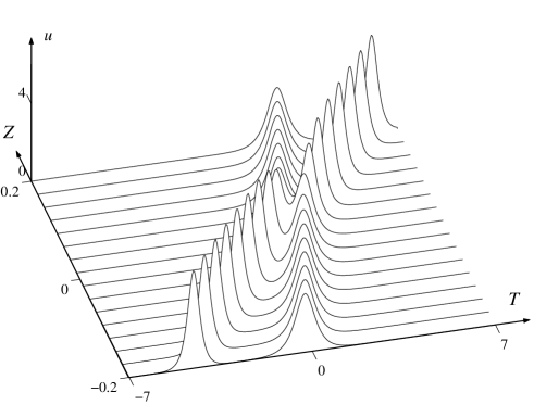
Figure 1: Two-soliton solution of the mKdV equation, using dimensionless parameters.

But expression (38) also describes the so-called higher order solitons, which can be considered as a pair of solitons of the above kind linked together, and have often an oscillatory behaviour. An example is given on figure 2. It uses the values of parameters $p_{1}=1+4i$, $p_{2}=p_{1}^{\ast}$, $\gamma_{1}=-\gamma_{2}=i\pi/2$. The corresponding spectrum is drawn on figure 3.

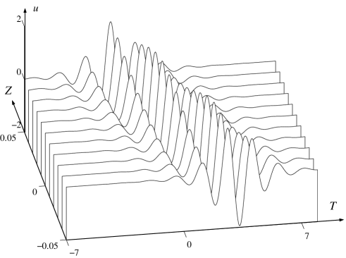
Figure 2: Second-order soliton solution of the mKdV equation, using dimensionless parameters.

Figure 3: (a) Pulse profile and (b) spectrum, of the second-order soliton solution of the mKdV equation of figure 2. Dimensionless parameters.

These spectrum and pulse profile are comparable to the experimental pulses given by [3]. It can thus be thought that the two-cycle pulses produced experimentally could propagate as solitons in certain media, according to the mKdV model.

4 Short-wave approximation

4.1 A sine-Gordon equation

We now consider the situation in which the resonance frequency $\Omega$ of the atoms is below the optical frequencies. Then the characteristic pulse duration $t_{w}$ is very small with regard to $t_{r}=2\pi/\Omega$, thus we use a short-wave approximation. We introduce a small perturbative parameter $\varepsilon$, such that the resonance period $t_{r}=\hat{t}_{r}/\varepsilon$, where $\hat{t}_{r}$ has the same order of magnitude as the pulse duration $t_{w}$. The perturbative parameter $\varepsilon$ is thus about $t_{w}/t_{r}$. Consequently, the Hamiltonian $H_{0}$ of the atom is replaced in the Schrödinger equation (6) by

$$\varepsilon\hat{H}_{0}.$$ (40)

We introduce a retarded time $\tau$ and a slow propagation variable $\zeta$ such that

$$\tau=\left(t-\frac{z}{V}\right)\quad,\quad\zeta=\varepsilon z.$$ (41)

The zero order reference time is chosen to be $t_{w}$, therefore $\tau$ is not a slow variable. The definition of the variable $\zeta$ gives account for long distance propagation. Computation shows that the dispersion effects arise at distances about $ct_{w}/\varepsilon$, from which follows the choice of the order of magnitude of $\zeta$. The electric field $E$ is expanded as $E=\sum_{n\geqslant 0}\varepsilon^{n}E_{n}$, and so on. The pulse duration $t_{w}$ is still assumed to be about one femtosecond, corresponding to an optical pulse of a few cycles. The relaxation times $\tau_{b}$, $\tau_{t}$ are very long with regard to $t_{w}$. Since the above scaling uses $t_{w}$ as zero-order reference time, this can be expressed by setting

$$\tau_{j}=\frac{\hat{\tau}_{j}}{\varepsilon}\quad\mbox{for $j=b$ and~{}$t$.}$$ (42)

Notice that (42) differs formally from the assumption (13) written in the previous section but represents the same physical hypothesis.

The above scaling can also be presented from another viewpoint, taking the characteristic time of the resonance $1/\Omega$ as zero-order reference time, as follows. The relevant component of the third order nonlinear susceptibility tensor $\chi^{(3)}$ computed from the above model is given by formula (27), where $\omega$ is the wave frequency (while $\Omega=\omega_{b}-\omega_{a}$ is the resonance frequency of the two-level system). The short-wave approximation corresponds to $\omega\longrightarrow\infty$. Then $\chi^{(3)}_{xxxx}$ tends to zero. Thus a linear behaviour of the wave can be expected in the short-wave approximation, except if the nonlinearity is very strong. The latter physical assumption can formally be expressed by assuming that the product $\mu E$ is very large with regard to $\Omega$, according to

$$H=H_{0}+\frac{1}{\varepsilon}\mu E,$$ (43)

where the small parameter $\varepsilon$ tends to zero. Then the short wave approximation can be sought using the expansions

$$\rho=\sum_{j\geqslant 0}\varepsilon^{j}\rho_{j}\quad,\quad E=\sum_{j\geqslant 0}\varepsilon^{j}E_{j}\quad,\quad P=\sum_{j\geqslant 0}\varepsilon^{j}P_{j},$$ (44)

and slow variables $\zeta$ and $\tau$ such that

$$\partial_{t}=\frac{1}{\varepsilon}\partial_{\tau}\quad,\quad\partial_{z}=\frac{-1}{\varepsilon V}\partial_{\tau}+\partial_{\zeta}.$$ (45)

The definition of variables (45) is very close to the standard short wave approximation formalism developed e.g. in [11, 12]. It is easily checked that the scalings (40-41) and (43-45) are equivalent. We refer to the former below.

The Schrödinger equation (6) at order $\varepsilon^{0}$ yields

$$i\partial_{\tau}\rho_{0a}=-E_{0}\left(\mu\rho_{0t}^{\ast}-\mu^{\ast}\rho_{0t}\right),$$ (46)

$$i\partial_{\tau}\rho_{0b}=+E_{0}\left(\mu\rho_{0t}^{\ast}-\mu^{\ast}\rho_{0t}\right),$$ (47)

$$i\partial_{\tau}\rho_{0t}=-E_{0}\mu\left(\rho_{0b}-\rho_{0a}\right).$$ (48)

From (46-47) we retrieve the normalization condition of the density matrix $\partial_{\tau}\mbox{tr}\,\rho=0$. We introduce the population inversion $w=\rho_{0b}-\rho_{0a}$ and get

$$\rho_{0}=\left(\begin{array}[]{cc}(\alpha-w)/2&i\mu\int^{\tau}E_{0}w\vspace{1.5mm}\\ -i\mu^{\ast}\int^{\tau}E_{0}w&(\alpha+w)/2\end{array}\right)$$ (49)

(as above, $\mbox{tr}\rho=\alpha=4\pi N\hbar c$ due to the normalization), and the equation

$$\partial_{\tau}w=-4|\mu|^{2}E_{0}\int^{\tau}E_{0}w.$$ (50)

Then expression (3) of the polarization $P$ yields $P_{0}=0$, and the Maxwell equation (4) at order $\varepsilon^{0}$ becomes trivial if the velocity is chosen as $V=1$.

The Schrödinger equation (6) at order $\varepsilon$ writes then as

$$i\partial_{\tau}\rho_{1}=\left[H_{0},\rho_{0}\right]-\left[\mu E_{0},\rho_{1}\right]-\left[\mu E_{1},\rho_{0}\right]+i\left(\begin{array}[]{cc}\rho_{0b}/{\tau_{b}}.&-\rho_{0t}/{\tau_{t}}\\ -\rho_{0t}^{*}/{\tau_{t}}&-\rho_{0b}/{\tau_{b}}\end{array}\right).$$ (51)

Defining $w_{1}=\rho_{1b}-\rho_{1a}$, the off-diagonal components of equation (51) yield

$$\rho_{1t}=i\left(\Omega+\frac{i}{\tau_{t}}\right)\int^{\tau}\rho_{0t}+i\mu\int^{\tau}(E_{0}w_{1}+E_{1}w),$$ (52)

so that the corresponding term $P_{1}=\mu^{\ast}\rho_{1t}+\mu\rho_{1t}^{\ast}$ of the polarization is

$$P_{1}=-2\Omega\left|\mu\right|^{2}\int^{\tau}\int^{\tau}Ew.$$ (53)

Notice again that the relaxation does not appear in the expression of the polarization at this order. The Maxwell equation (4) at order $\varepsilon$ then reduces to

$$\partial_{\zeta}\partial_{\tau}E_{0}=\Omega|\mu|^{2}E_{0}w\;.$$ (54)

Equations (50,54) yield the sought system. If we set

$$p=-i|\mu|^{2}\int^{\tau}E_{0}w,$$ (55)

they reduce to

$$\partial_{\zeta}E_{0} = i\Omega p,$$ (56)

$$\partial_{\tau}p = -i|\mu|^{2}E_{0}w,$$ (57)

$$\partial_{\tau}w = -4iE_{0}p,$$ (58)

which coincide with the equations of the self-induced transparency, although the physical situation is quite different: the characteristic frequency $1/t_{w}$ of the pulse is far above the resonance frequency $\Omega$, while the self-induced transparency occurs when the optical field oscillates at the frequency $\Omega$. The quantities $E$ and $w$ describe here the electric field and population inversion themselves, and not amplitudes modulating a carrier with frequency $\Omega$. Notice that $E$ and $w$ are here real quantities, and not complex ones as in the case of the self-induced transparency. Further, $p$ is not the polatization density, but is proportional to its $\tau$-derivative. Another difference is the absence of a factor $1/2$ in the right-hand side of equation (56).

Since they explicitly involve the population inversion, the model equations (56-58) cannot be generalized easily to more realistic situation in which an arbitrary number of atomic levels are taken into account. Recall that, according to the assumption made at the beginning of the section, this model is valid for a very strong nonlinearity only. In particular, we assumed that the atomic dipolar momentum $\mu$ has a very large value. In a more realistic situation, it can be expected that only the transition corresponding to the largest value of the dipolar momentum will have a significant contribution. If several transitions correspond to large values of the dipolar momentum with the same order of magnitude, we can expect that the short-wave approximation will yield some more complicated asymptotic system involving the populations of each level concerned. The derivation of such a model is left for further study.

4.2 The two-soliton solution

Using dimensionless variables defined by

$$\Theta=\frac{E_{0}}{E_{r}}\quad,\quad W=\frac{w}{w_{r}}\quad,\quad T=\frac{\tau}{T_{0}}\quad,\quad Z=\frac{\zeta}{L},$$ (59)

where the reference values satisfy

$$E_{r}T_{0}|\mu|=1\quad\mbox{and}\quad w_{r}L\Omega T_{0}|\mu|^{2}=2,$$ (60)

and setting $\eta=\int^{Z}W$, the system (50-54) reduces to

$$\partial_{Z}\partial_{T}\Theta = 2\Theta\partial_{Z}\eta,$$ (61)

$$\partial_{Z}\partial_{T}\eta = -2\Theta\partial_{Z}\Theta.$$ (62)

Equations (61-62) have been found to describe short electromagnetic wave propagation in ferrites, using the same kind of short-wave approximation [11].

The following change of dependant variables:

$$\partial_{Z}\eta = A\cos u,$$ (63)

$$\partial_{Z}\Theta = A\sin u,$$ (64)

transforms equations (61-62) into [11, 13]

$$\partial_{T}A = 0,$$ (65)

$$\partial_{Z}\partial_{T}u = 2A\sin u.$$ (66)

Since, according to (65), $A$ is a constant, (66) is the sine-Gordon equation. Before we recall some properties of the latter, let us determine the physical meaning of the constant $A$ in the present physical frame. Using relations (63-64) and the definition of $\eta$, we find that

$$A^{2}=\lim_{T\longrightarrow\infty}\left(W^{2}+\left(\partial_{Z}\Theta\right)^{2}\right)$$ (67)

Since $\Theta$ is the dimensionless wave electric field, it vanishes at infinity. Thus we can have a non-vanishing solution only if some initial population inversion $w_{i}=W_{i}w_{r}$ is present. The constant involved by equation (66) is then $A=W_{i}$.

Using the variable ${\hat{Z}}=2W_{i}Z$, equation (66) reduces to the sine-Gordon equation

$$\partial_{\hat{Z}}\partial_{T}u=\sin u.$$ (68)

The quantities involved by equation (68) are related to the quantities measured in the laboratory through

$$\hat{Z}=\frac{z}{\hat{L}}\quad,\quad T=\frac{1}{t_{w}}\left(t-\frac{z}{c}\right),$$ (69)

$$E=\frac{E_{r}}{2}\int^{\hat{Z}}\sin u\quad,\quad w=w_{i}\cos u.$$ (70)

The electric field and propagation length scaling parameters are

$$E_{r} = \frac{\hbar}{|\mu|t_{w}},$$ (71)

$$\hat{L} = \frac{\hbar c}{\Omega t_{w}4\pi N|\mu|^{2}w_{i}},$$ (72)

in which the initial population inversion $w_{i}$ and typical pulse duration $t_{w}$ are given. The small perturbative parameter $\varepsilon$ can be identified with $\Omega t_{w}$, expressing the fact that $t_{w}$ is very small with regard to $1/\Omega$.

The sine-Gordon equation (68) is completely integrable [13]. A $N$-soliton solution can be found using either the IST or the Hirota method. As in section 2, we will consider here the two-soliton solution only, which is [13]

$$u=2i\ln\left(\frac{f^{\ast}}{f}\right),$$ (73)

with

$$f=1+ie^{\eta_{1}}+ie^{\eta_{2}}-\frac{(k_{1}-k_{2})^{2}}{(k_{1}+k_{2})^{2}}e^{\eta_{1}+\eta_{2}},$$ (74)

where

$$\eta_{j}=k_{j}T+\frac{Z}{k_{j}}+\gamma_{j}\quad\mbox{for $j=1$, $2$,}$$ (75)

$k_{1}$, $k_{2}$, $\gamma_{1}$ and $\gamma_{2}$ being arbitrary parameters. When they take real values, formulas (73-75) describe the interaction of two solitons. The behaviour is very close to that of the typical two-soliton solution of the mKdV equation shown in figure 1. As in the case of the long wave approximation, the two-soliton solution (73-75) is also able to describe soliton-type propagation of a pulse in the two-cycle regime. The corresponding analytic solution is a second-order soliton or breather, which can be considered as two bounded solitons, and is obtained using complex conjugate values of the soliton parameters $k_{1}$ and $k_{2}$. An example is given in figure 4, with the values of parameters $k_{1}=1+4i$, $k_{2}=1-4i$, $\gamma_{1}=\gamma_{2}=0$.

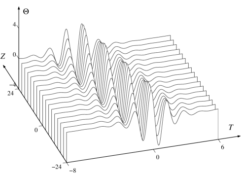
Figure 4: Electric field evolution of the second-order soliton solution of the sine-Gordon equation, using dimensionless parameters.

The pulse profile, with the corresponding population inversion and spectrum are drawn in figure 5. The profile and spectrum are comparable with the experimental observation of [3].

Figure 5: (a) Pulse profile, (b) population inversion and (c) spectrum, of the second-order soliton solution of the sine-Gordon equation of figure 4. Dimensionless parameters.

Notice again that an initial population inversion $w_{i}\neq 0$ is required. Total inversion ($w_{i}=1$) is not necessary but, as shows the expression (72) of the propagation reference length $\hat{L}$, a small inversion reduces the soliton amplitude and increases the propagation distance at which nonlinear effects occur.

5 Conclusion

We have given two models that allow the description of ultrashort optical pulses propagation in a medium described by a two-level Hamiltonian, when the slowly varying envelope approximation cannot be used. Using approximations based on the hypothesis that the resonance frequency of the medium is far from the field frequency, we derived completely integrable models. When the resonance frequency is well above the inverse of the typical pulse width of about one femtosecond, a long-wave approximation leads to a mKdV equation. When in the contrary the resonance frequency is well below the field frequency, a short-wave approximation leads to a model formally identical to that describing self-induced transparency, but in very different validity conditions. It can be reduced to the sine-Gordon equation. The scaling parameters for these approximations have been written down explicitly.

Both the mKdV and the sine-Gordon equations are completely integrable by means of the IST method and admit $N$-soliton solutions. The two-soliton solution is able to describe the propagation of a pulse in the two-cycle regime, very close in shape and spectrum to the pulses of this type produced experimentally. It does not mean that the formulas of this paper describe the experimental results, because we have considered a propagation problem, and experimental results concern pulses generated directly at the laser output. But we have shown that soliton-type propagation, with only periodic deformation of the pulse during the propagation, may occur for such type of pulses, under adequate conditions. In the short-wave approximation, these conditions involve an initial population inversion, at least a partial one.

Further, the study of a two-level Hamiltonian can be considered as an academic problem, showing the tractability of such an approach. A rather remarkable feature is that the computations involved by the derivation of the asymptotic models are relatively short and easy. Therefore the application of the same approach to more realistic situations can be reasonably envisaged. A generalization of the mKdV equation obtained in the long-wave approximation has been proposed on heuristic grounds, and should be justified rigorously. A generalization of the model obtained in the short-wave approximation would require a special study. Last, in a more realistic model, it can be envisaged that some transition frequencies are well above the inverse of the characteristic pulse duration, but that some other are below it. The treatment of such a situation will mix the above short-wave and long-wave approximations, it is left for further study. It can be expected that the result will depend strongly on the particular physical situation considered.

References

- [1] D.H. Sutter, G. Steinmeyer, L. Gallmann, N. Matuschek, F. Morier-Genoud, U. Keller, V. Scheuer, G. Angelow, and T. Tschudi, Semiconductor saturable-absorber mirror-assisted Kerr-lens mode-locked Ti:sapphire laser producing pulses in the two-cycle regime Opt. Lett. 24 (9) 631-633 (1999).
- [2] U. Morgner, F.X. Kärtner, S.H. Cho, Y. Chen, H.A. Haus, J.G. Fujimoto, E.P. Ippen, V. Scheuer, G. Angelow, and T. Tschudi, Sub-two-cycle pulses from a Kerr-lens mode-locked Ti:sapphire laser, Opt. Lett. 24 (6) 411-413 (1999).
- [3] R. Ell, U. Morgner, F.X. Kärtner, J.G. Fujimoto, E.P. Ippen, V. Scheuer, G. Angelow, T. Tschudi, M.J. Lederer, A. Boiko, and B. Luther-Davies, Generation of 5-fs pulses and octave-spanning spectra directly from a Ti:sapphire laser, Opt. Lett. 26 (6) 373-375 (2001).
- [4] S. Blair, Non-paraxial 1-D spatial solitons, Chaos 10, 570 (2000).
- [5] A.I. Smirnov and A.A. Zharov, Nonparaxial solitons, in: A.D. Boardman and A.P. Sukhorukov (eds.), Soliton-driven Photonics, NATO Science Series (Kluwer, Dordrecht, 2001).
- [6] T. Taniuti et C.-C. Wei, Reductive perturbation method in nonlinear wave propagation I, J. Phys. Soc. Japan, 24, 941-946 (1968).
- [7] H. Leblond, Higher order terms in multiscale expansions: A linearized KdV Hierarchy, Journal of Nonlinear Mathematical Physics 9 (3) 325-346 (2002).
- [8] R.W. Boyd, Nonlinear Optics (Academic Press inc., San Diego, 1992)
- [9] M. Wadati, The modified Korteweg-de Vries equation, J. Phys. Soc. Jpn. 34 (5), 1289-1296 (1973).
- [10] R. Hirota, Direct method of finding exact solutions of nonlinear evolution equations. Bäcklund transformations, the inverse scattering method, solitons, and their applications (Workshop Contact Transformation, Vanderbilt Univ., Nashville, Tenn., 1974), pp 40-68, Lecture Notes in Math. 515, Springer, Berlin, 1976.
- [11] R.A. Kraenkel, M.A. Manna, and V. Merle, Nonlinear short-wave propagation in ferrites, Phys. Rev. E, 61 (1), 976-979 (2000).
- [12] M.A. Manna, Asymptotic dynamics of monochromatic short surface wind waves, Physica D 149, 231-236 (2001).
- [13] M.J. Ablowitz and H. Segur, Solitons and the Inverse Scattering Transform, SIAM, Philadelphia (1981).