Fine structure of distributions and central limit theorem in diffusive billiards

Abstract

We investigate deterministic diffusion in periodic billiard models, in terms of the convergence of rescaled distributions to the limiting normal distribution required by the central limit theorem; this is stronger than the usual requirement that the mean square displacement grow asymptotically linearly in time. The main model studied is a chaotic Lorentz gas where the central limit theorem has been rigorously proved. We study one-dimensional position and displacement densities describing the time evolution of statistical ensembles in a channel geometry, using a more refined method than histograms. We find a pronounced oscillatory fine structure, and show that this has its origin in the geometry of the billiard domain. This fine structure prevents the rescaled densities from converging pointwise to gaussian densities; however, demodulating them by the fine structure gives new densities which seem to converge uniformly. We give an analytical estimate of the rate of convergence of the original distributions to the limiting normal distribution, based on the analysis of the fine structure, which agrees well with simulation results. We show that using a Maxwellian (gaussian) distribution of velocities in place of unit speed velocities does not affect the growth of the mean square displacement, but changes the limiting shape of the distributions to a non-gaussian one. Using the same methods, we give numerical evidence that a non-chaotic polygonal channel model also obeys the central limit theorem, but with a slower convergence rate.

I Introduction

Diffusion, the process by which concentration gradients are smoothed out, is one of the most fundamental mechanisms in physical systems out of equilibrium. Understanding the microscopic processes which lead to diffusion on a macroscopic scale is one of the goals of statistical mechanics Dorfman (1999). Since Einstein’s seminal work on Brownian motion Gardiner (1985), diffusion has been modeled by random processes. However, we expect the microscopic dynamics to be described by deterministic equations of motion.

Recently it has been realized that many simple deterministic dynamical systems are diffusive in some sense; we call this deterministic diffusion. Such systems can be regarded as toy models to understand transport processes in more realistic systems Dorfman (1999). Examples include classes of uniformly hyperbolic one-dimensional (1D) maps (see e.g. Klages and Dorfman (1999) and references therein) and multibaker models Gaspard (1998). Often rigorous results are not available, but numerical results and analytical arguments indicate that diffusion occurs, for example in hamiltonian systems such as the standard map Lichtenberg and Lieberman (1992).

Billiard models, where non-interacting point particles in free motion undergo elastic collisions with an array of fixed scatterers, have been particularly studied, since they are related to hard sphere fluids, while being amenable to rigorous analysis Bunimovich and Sinai (1980/81); Bunimovich et al. (1991); Gaspard (1998). They can also be regarded as the simplest physical systems in which diffusion, understood as the large-scale transport of mass through the system, can occur Bunimovich (2000). In this paper we study deterministic diffusion in two 2D billiard models: a periodic Lorentz gas, where the scatterers are disjoint disks, and a polygonal billiard channel.

A definition often used in the physical literature is that a system is diffusive if the mean square displacement grows proportionally to time $t$, asymptotically as $t\to\infty$. However, there are stronger properties which are also characteristic of diffusion, which a given system may or may not possess: (i) a central limit theorem may be satisfied, i.e. rescaled distributions converge to a normal distribution as $t\to\infty$; and (ii) the rescaled dynamics may ‘look like’ Brownian motion.

Two-dimensional (2D) periodic Lorentz gases were proved in Bunimovich and Sinai (1980/81); Bunimovich et al. (1991) to be diffusive in these stronger senses if they satisfy a geometrical finite horizon condition (Sec. II.1). We use a square lattice with an additional scatterer in each cell to satisfy this condition, a geometry previously studied in Garrido and Gallavotti (1994); Garrido (1997). This model is of interest since, unlike in the commonly studied triangular lattice case (see e.g. Gaspard (1998); Machta and Zwanzig (1983); Klages and Dellago (2000)), we can vary independently two physically relevant quantities: the available volume in a unit cell, and the size of its exits; this is possible due to the two-dimensional parameter space Sanders ; Sanders (2004).

The main focus of this paper is to investigate the fine structure occurring in the position and displacement distributions at finite time $t$, and the relation with the convergence to a limiting normal distribution as $t\to\infty$ proved in Bunimovich and Sinai (1980/81); Bunimovich et al. (1991). Those papers show in what sense we can smooth away the fine structure to obtain convergence. However, from a physical point of view it is important to understand how this convergence occurs; our analysis provides this.

This analysis makes explicit the obstruction that prevents a stronger form of convergence, showing how density functions fail to converge pointwise to gaussian densities; it also allows us to conjecture a more refined result which takes the fine structure into account.

Furthermore, this line of argument suggests how convergence may occur in other models where few rigorous results are available. As an example, we analyze a recently-introduced polygonal billiard channel model, showing that the same techniques are still applicable.

Plan of paper

In Sec. II we present the periodic Lorentz gas model for which we obtain most of our results. Section III discusses the definition of diffusion in the context of deterministic dynamical systems. In Sec. IV we study numerically the fine structure of distributions in the Lorentz gas, finding good agreement with an analytical calculation in terms of the geometry of the billiard domain, and showing that when this fine structure is removed, the demodulated densities are close to gaussian. This we apply in Sec. V to investigate the central limit theorem and the rate of convergence to the limiting normal distribution, obtaining a simple estimate of this rate which agrees well with numerical results. In Sec. VI we study the effect of imposing a Maxwellian (gaussian) velocity distribution in place of a unit speed distribution, showing that this leads to non-gaussian limiting distributions. Section VII extends these ideas to a polygonal billiard channel, where few rigorous results are available. We finish with conclusions in Sec. VIII.

II Two-dimensional periodic Lorentz gas

We consider periodic billiard models, where the dynamics can be studied on the torus. The region $Q$ exterior to the scatterers is called the billiard domain; we denote its area by $\left|Q\right|$. Since the particles are non-interacting, it is usual to set all velocities to $1$ by a geometrical rescaling, although in Sec. VI we discuss the effect of a gaussian velocity distribution.

We focus on a periodic Lorentz gas, where the scatterers are non-overlapping disks. Their strictly convex boundaries make this a scattering billiard Bunimovich and Sinai (1980/81), and hence a chaotic system, in the sense that it has a positive Lyapunov exponent Chernov and Markarian (2001); Gaspard (1998) and positive Kolmogorov–Sinai entropy Gaspard (1998).

II.1 Periodic Lorentz gas model

The model we study, previously considered in Garrido and Gallavotti (1994); Garrido (1997), consists of two square lattices of disks; they have the same lattice spacing $r$, and radii $a$ and $b$, respectively, and are positioned such that there is a $b$-disk at the center of each unit cell of the $a$-lattice: see Fig. 1. In analytical calculations we take the length scale as $r=1$, as in Garrido (1997); Garrido and Gallavotti (1994), whereas in numerical simulations we fix $a=1$ and scale $r$ and $b$ appropriately, as in Klages and Dellago (2000).

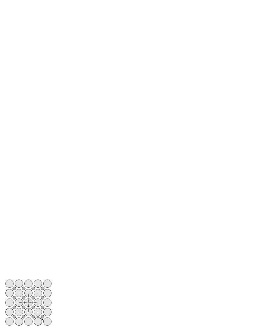
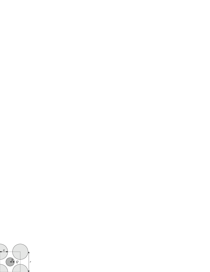
Figure 1: (a) Part of the infinite system, constructed from two square lattices of disks shown in different shades of gray; dashed lines indicate several unit cells and an elastic collision is shown. (b) A single unit cell, defining the geometrical parameters. The billiard domain is the area $Q$ exterior to the disks.

Finite horizon condition

Periodic Lorentz gases were shown in Bunimovich and Sinai (1980/81); Bunimovich et al. (1991) to be diffusive (Sec. III), provided they satisfy the finite horizon condition: there is an upper bound on the free path length between collisions. If this is not the case, so that a particle can travel infinitely far without colliding (the billiard has an infinite horizon), then corridors exist Bleher (1992), which allow for fast propagating trajectories, leading to super-diffusive behavior, as was recently rigorously proved Szász and Varjú (2003).

We restrict attention to parameter values within the finite horizon regime by choosing $b$ to block all corridors Garrido (1997); Sanders .

II.2 Statistical properties

Statistical properties of deterministic dynamical systems arise from an ensemble of initial conditions $(\mathbf{x}_{0},\mathbf{v}_{0})$ modeling the imprecision of physical measurements. We always take a uniform distribution with respect to Liouville measure in one unit cell: the positions $\mathbf{x}_{0}$ are uniform with respect to Lebesgue measure in the billiard domain $Q$, and the velocities $\mathbf{v}_{0}$ are uniform in the unit circle $S^{1}$, i.e. with angles between $0$ and $2\pi$, and unit speeds.

We evolve $(\mathbf{x}_{0},\mathbf{v}_{0})$ for a time $t$ under the billiard flow $\Phi^{t}$ in phase space to $(\mathbf{x}(t),\mathbf{v}(t))$. Note that Liouville measure on the torus is invariant under this flow Chernov and Markarian (2001). In numerical experiments, we take a large sample $(\mathbf{x}^{(i)}_{0},\mathbf{v}^{(i)}_{0})_{i=1}^{N}$ of size $N$ of initial conditions chosen uniformly with respect to Liouville measure using a random number generator. These evolve after time $t$ to $(\mathbf{x}^{(i)}(t),\mathbf{v}^{(i)}(t))_{i=1}^{N}$; the distribution of this ensemble then gives an approximation to that of $(\mathbf{x}(t),\mathbf{v}(t))$.

We denote averages over the initial conditions, or equivalently expectations with respect to the distribution of $(\mathbf{x}_{0},\mathbf{v}_{0})$, by $\langle\cdot\rangle$. Approximations of such averages can be evaluated using a simple Monte Carlo method Press et al. (1992) as

$$\langle f(\mathbf{x}_{0},\mathbf{v}_{0})\rangle=\lim_{N\to\infty}\frac{1}{N}\sum_{i=1}^{N}f(\mathbf{x}_{0}^{(i)},\mathbf{v}_{0}^{(i)}).$$ (1)

The infinite sample size limit, although unobtainable in practice, reflects the expectation that larger $N$ will give a better approximation. Averages at time $t$ can be evaluated by using a function $f$ involving $\Phi^{t}$.

II.3 Channel geometry

Diffusion occurs in the extended system obtained by unfolding the torus to a 2D infinite lattice: see Bunimovich and Sinai (1980/81); Bunimovich et al. (1991) and Sec. III. The diffusion process is then described by a second order diffusion tensor having $4$ components $D_{ij}$ with respect to a given orthonormal basis, given by

$$D_{ij}=\lim_{t\to\infty}\frac{1}{2t}\langle\Delta x_{i}\Delta x_{j}\rangle_{t}.$$ (2)

The square symmetry of our model reduces the diffusion tensor to a constant multiple $D$ of the identity tensor; we can evaluate this diffusion coefficient by restricting attention to the dynamics in a $1$-dimensional channel extended only in the $x$-direction; see Fig. 2. Correspondingly, we restrict attention to 1D marginal distributions.

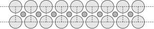
Figure 2: 1D channel obtained by unfolding torus in $x$-direction.

A channel geometry, with hard horizontal boundaries, corresponding to the triangular Lorentz gas was studied in Gaspard (1993); Alonso et al. (1999) (Fig. 3). This is equivalent to a channel with twice the original height and periodic boundaries, shown in Fig. 3 as part of the whole triangular lattice obtained by unfolding completely in the vertical direction. We can view this lattice as consisting of rectangular unit cells (Fig. 3) which are stretched versions of the square unit cell considered above, with the extra condition $a=b$. The results in the remainder of this paper then extend to this case with minor changes.

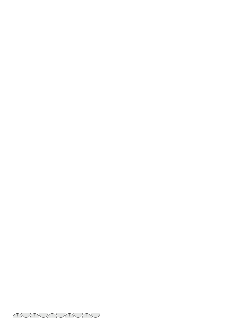
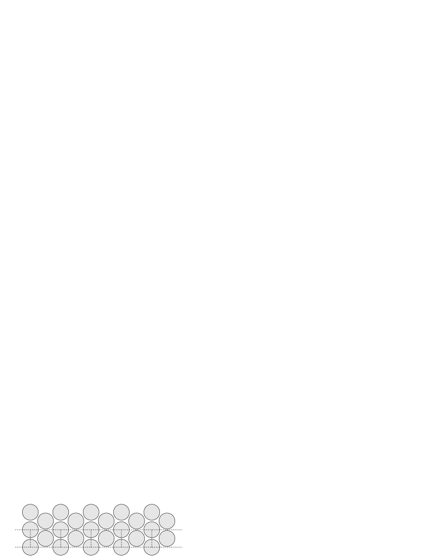
Figure 3: (a) Lorentz channel studied in Gaspard (1993); Alonso et al. (1999) with hard upper and lower boundaries; dotted lines indicate unit cells. (b) Fully unfolded triangular Lorentz gas. Dotted lines indicate unit cells forming a channel with periodic upper and lower boundaries.

III Deterministic diffusion

In this section we briefly recall how to make precise the fact that the behavior of certain deterministic dynamical systems ‘looks like’ that of the diffusion equation.

III.1 Diffusion as a stochastic process

Diffusion is described classically by the diffusion equation

$$\frac{\partial\rho(t,\mathbf{x})}{\partial t}=D\,\nabla^{2}\rho(t,\mathbf{x}),$$ (3)

where $\rho$ is the density of the diffusing substance. Following Einstein and Wiener (see e.g. Gardiner (1985)), we can model diffusion as a stochastic process $B_{t}$, determined by the probability density $p(\mathbf{x},t)$ of a particle being at position $\mathbf{x}$ at time $t$ given that it started at $\mathbf{x}=\mathbf{0}$ at time $t=0$.

Imposing conditions on the process determined from physical requirements gives a diffusion process, where $p(\mathbf{x},t)$ satisfies the equation

$$\frac{\partial p}{\partial t}+\frac{\partial}{\partial x_{i}}\left[A_{i}\,p-\frac{1}{2}\sum_{j}\frac{\partial}{\partial x_{j}}\left(B_{ij}\,p\right)\right]=0,$$ (4)

known as Kolmogorov’s forward equation or the Fokker–Planck equation Gardiner (1985). The drift vector $\mathbf{A}(\mathbf{x},t)$ and the diffusion tensor $\mathsf{B}(\mathbf{x},t)$ give the mean and variance, respectively, of infinitesimal displacements at position $\mathbf{x}$ and time $t$ Gardiner (1985).

If the system is sufficiently symmetric that the drift is zero and the diffusion tensor is a multiple of the identity tensor, then the process is Brownian motion, and (4) reduces to the diffusion equation (3). A general diffusion process, however, can be inhomogeneous in both space and time.

III.2 Diffusion in dynamical systems via limit theorems

Diffusion in billiards concerns the statistical behavior of the particle positions. We can write the first component $x_{t}$ of the position $\mathbf{x}_{t}$ at time $t$ as

$$x_{t}=\int_{0}^{t}v_{1}(s)\,\textrm{d}s+x_{0}=\int_{0}^{t}f\circ\Phi^{s}(\cdot)\,\textrm{d}s+x_{0},$$ (5)

where $f=v_{1}$, the first velocity component. This expresses $x_{t}$ solely in terms of functions defined on the torus. In fact, (5) shows that the displacement $\Delta x_{t}:=x_{t}-x_{0}$ is in some sense a more natural observable than the position $x_{t}$ in this context.

We thus wish to study the distribution of accumulation functions of the form $S_{t}(\cdot):=\int_{0}^{t}f\circ\Phi^{s}(\cdot)\,\textrm{d}s$, in particular in the limit as $t\to\infty$ Chernov and Young (2000). We remark that other observables $f$ are relevant for different transport processes Bunimovich (2000).

We denote by $\Phi^{t}\colon\mathcal{M}\to\mathcal{M}$ the flow of a dynamical system with time $t\in\mathbb{R}$. Given a probability measure $\mu$ describing the distribution of initial conditions, we can find the probability of being in certain regions of the phase space $\mathcal{M}$ at given times, so that we have a stochastic process. If the measure $\mu$ is invariant, so that $\mu(\Phi^{-t}(A))=\mu(A)$ for all times $t$ and all nice sets $A$, then the stochastic process is stationary Chernov and Young (2000).

The integral in the definition of $S$ is then a continuous-time version of a Birkhoff sum $\sum_{i=0}^{n-1}f\circ\Phi^{i}$ over the stationary stochastic process given by $\Phi$, so that we may be able to apply limit theorems from the theory of stationary stochastic processes Chernov and Young (2000). For the case of the periodic Lorentz gas with finite horizon, it was proved in Bunimovich and Sinai (1980/81); Bunimovich et al. (1991) that the following limit theorems hold.

Asymptotic linearity of mean square displacement

The limit

$$2D:=\lim_{t\to\infty}\frac{1}{t}\langle\Delta x^{2}\rangle_{t}$$ (6)

exists, so that the mean square displacement $\langle\Delta x^{2}\rangle_{t}:=\langle\left[\Delta x(t)\right]^{2}\rangle$ (the variance of the displacement distribution) grows asymptotically linearly in time:

$$\langle\Delta x^{2}\rangle_{t}\sim 2Dt\quad\text{as }t\to\infty,$$ (7)

where $D$ is the diffusion coefficient. In $d\geq 2$ dimensions, setting $\Delta x_{i}(t):=x_{i}(t)-x_{i}(0)$, we have

$$\langle\Delta x_{i}\,\Delta x_{j}\rangle_{t}\sim 2D_{ij}t,$$ (8)

where the $D_{ij}$ are components of a symmetric diffusion tensor.

Central limit theorem: convergence to normal distribution

Scale the displacement distribution by $\sqrt{t}$, so that the variance of the rescaled distribution is bounded. Then this distribution converges weakly, or in distribution, to a normally distributed random variable $\mathbf{z}$ Gaspard and Nicolis (1990); Chernov and Young (2000):

$$\frac{\mathbf{x}(t)-\mathbf{x}(0)}{\sqrt{t}}\stackrel{{\scriptstyle\mathcal{D}}}{{\longrightarrow}}\mathbf{z},\qquad\text{as }t\to\infty.$$ (9)

In the $1$-dimensional case, this means that

$$\lim_{t\to\infty}\mathbb{P}\left(\frac{x_{t}-x_{0}}{\sqrt{t}}<u\right)=\frac{1}{\sigma\sqrt{2\pi}}\int_{s=-\infty}^{u}\mathrm{e}^{-s^{2}/2\sigma^{2}}\,\textrm{d}s,$$ (10)

where $\mathbb{P}(\cdot)$ denotes probability with respect to the distribution of the initial conditions, and $\sigma^{2}$ is the variance of the limiting normal distribution. In $d\geq 2$ dimensions, this is replaced by similar statements about probabilities of $d$-dimensional sets. This is the central limit theorem for the random variable $\Delta x$. From (a) we know that in 1D, the variance of the limiting normal distribution is $\sigma^{2}=2D$; in $d\geq 2$ dimensions, the covariance matrix of $\mathbf{z}$ is given by the matrix $(2D_{ij})$ Bunimovich and Sinai (1980/81); Dettmann and Cohen (2000).

Functional central limit theorem: convergence of path distribution to Brownian motion

We rescale the path $\mathbf{x}_{t}$ by the scale from (b), defining $\tilde{\mathbf{x}}_{t}$ by Bleher (1992)

$$\tilde{\mathbf{x}}_{t}(s):=\frac{\mathbf{x}(st)-\mathbf{x}(0)}{\sqrt{t}},\quad s\in[0,1].$$ (11)

The distribution of these rescaled paths then converges in distribution to Brownian motion:

$$\tilde{\mathbf{x}}_{t}\stackrel{{\scriptstyle\mathcal{D}}}{{\longrightarrow}}\mathbf{B}\quad\text{as }t\to\infty,$$ (12)

where the Brownian motion $\mathbf{B}$ has covariance matrix as in (b). This is known as a functional central limit theorem, or weak invariance principle Chernov and Young (2000).

A sufficient condition for this is that the following two properties hold Billingsley (1968). (i) The multi-dimensional central limit theorem, a generalization of (b), is satisfied. This says that the finite-dimensional distributions of the process $\tilde{\mathbf{x}}_{t}$ converge to those of Brownian motion, so that for any $n$, any times $s_{1}<\cdots<s_{n}$, and any reasonable sets $D_{1},\ldots,D_{n}$ in $\mathbb{R}^{d}$, we have

$$\mathbb{P}\left(\tilde{\mathbf{x}}_{t}(s_{1})\in D_{1},\ldots,\tilde{\mathbf{x}}_{t}(s_{n})\in D_{n}\right)\\ \stackrel{{\scriptstyle t\to\infty}}{{\longrightarrow}}\mathbb{P}\left(\mathbf{B}(s_{1})\in D_{1},\ldots,\mathbf{B}(s_{n})\in D_{n}\right).$$ (13)

The right-hand side can be expressed as a multi-dimensional integral over gaussians: see e.g. Dettmann and Cohen (2000); Sanders (2004). (ii) The convergence is tight, which prevents mass escaping to infinity: see Billingsley (1968) for the definition.

III.3 Discussion of definitions of diffusion

Property (c) is the strongest sense in which a dynamical system can show deterministic diffusion, making precise how a rescaled dynamical system can look like Brownian motion. However, few physically relevant systems have been proved to satisfy (c): interest in the periodic Lorentz gas comes largely from the fact that it is one; another is the triple linkage Hunt and MacKay (2003).

The multi-dimensional central limit theorem part of (c) was studied in Dettmann and Cohen (2000), where both Lorentz gases and wind–tree models were found to obey it, tested for certain sets $D_{i}$ and certain values of $n$. However, as stated in Dettmann and Cohen (2000), (c) is difficult to investigate numerically, and the results in that paper seem to be the best that we can expect.

Property (b), the central limit theorem, has been shown for large classes of observables $f$ in many dynamical systems (see Chernov and Young (2000) and references therein), but again they are often not physical. Property (b) was used in Gaspard and Nicolis (1990) as the definition of a diffusive system, but does not seem to have been applied in the physical literature; it is the approach taken in this paper.

Many papers in the physical literature define a system to be diffusive if only property (a) is verified (numerically), e.g. Klages and Dellago (2000); Alonso et al. (2002); Dettmann and Cohen (2001). Many types of system are diffusive in this sense, including 1D maps Klages and Dorfman (1999), random Lorentz gases Dettmann and Cohen (2001) and Ehrenfest wind–tree models, both periodic Alonso et al. (2002) and random Dettmann and Cohen (2001).

It is possible for the weaker properties to hold when the stronger ones do not. For example, in Kong and Cohen (1989) a disordered lattice-gas wind–tree model was reported to have an asymptotically linear mean square displacement, but a non-gaussian distribution function, i.e. (a) but not (b). However, disorder can lead to trapping effects which cannot occur in periodic systems Alonso et al. (2002), and we are not aware of a periodic (and hence ordered) billiard-type model with unit-speed velocity distribution which shows (a) but not (b), although in Sec. VI we show that this can occur with a Maxwellian velocity distribution.

IV Fine structure of position and displacement distributions

We now focus on the diffusive properties of the periodic Lorentz gas model introduced in Sec. II. In this section, we describe the fine structure of position and displacement distributions. The displacement distribution occurs naturally in the central limit theorem (Sec. III.2) and in Green–Kubo relations Dorfman (1999); Gaspard (1998), whereas the position distribution is more natural if we are unable to track the paths of individual particles. It is possible to show that the asymptotic properties of the position and displacement distributions are the same, in the sense that one has an asymptotically linear growth if and only if the other does, and similarly for the central limit theorem Sanders (2004). It is hence equivalent to consider diffusive properties by studying either distribution.

IV.1 Position and displacement distributions

Figure 4 shows scatterplots representing 2D position and displacement distributions for a representative choice of geometrical parameters. Each dot represents one initial condition started in the central unit cell and evolved for time $t=50$; $N=5\times 10^{4}$ samples are shown. Both distributions show decay away from a maximum in the central cell, an overall circular shape, and the occurrence of a periodic fine structure.

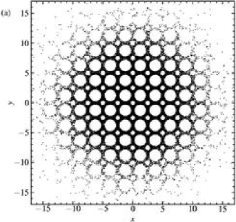
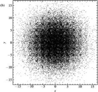
Figure 4: (a) 2D position distribution; (b) 2D displacement distribution. $r=2.5$; $b=0.4$; $t=50$; $N=5\times 10^{4}$ initial conditions.

These figures are projections to the billiard domain $Q$ of the density in the phase space $Q\times S^{1}$. Since the dynamics on the torus is mixing Chernov and Markarian (2001), the phase space density converges weakly Lasota and Mackey (1994) to a uniform density on phase space corresponding to the invariant Liouville measure. Physically, the phase space density develops a complicated layer structure in the stable direction of the dynamics: see e.g. Dorfman (1999). Projecting corresponds to integrating over the velocities; we expect this to eliminate this complicated structure and result in some degree of smoothness of the projected densities. However, we are not aware of any rigorous results in this direction, even for relatively well-understood systems such as the Arnold cat map Dorfman (1999).

These 2D distributions are difficult to work with, and we instead restrict attention to one-dimensional marginal distributions, i.e. projections onto the $x$-axis, which will also have some degree of smoothness. We denote the 1D position density at time $t$ and position $x\in\mathbb{R}$ by $f_{t}(x)$ and the displacement density for displacement $x$ by $g_{t}(x)$. We let their respective (cumulative) distribution functions be $F_{t}(x)$ and $G_{t}(x)$, respectively, so that

$$F_{t}(x):=\mathbb{P}(x_{t}\leq x)=\int_{-\infty}^{x}f_{t}(s)\,\textrm{d}s,\\$$ (14)

and similarly for $G_{t}$. (When necessary, we will instead denote displacements by $\xi$.) The densities show the structure of the distributions more clearly, while the distribution functions are more directly related to analytical considerations.

IV.2 Numerical estimation of distribution functions and densities

We wish to estimate numerically the above denstities and distribution functions at time $t$ from the $N$ data points $x_{t}^{(1)},\ldots,x_{t}^{(N)}$. The most widely used method in the physics community for estimating density functions from numerical data is the histogram; see e.g. Alonso et al. (2002). However, histograms are not always appropriate, due to their non-smoothness and dependence on bin width and position of bin origin Silverman (1986). In Alonso et al. (2002), for example, the choice of a coarse bin width obscured the fine structure of the distributions that we describe in Sec. VII.

We have chosen the following alternative method, which seems to work well in our situation, since it is able to deal with strongly peaked densities more easily, although we do not have any rigorous results to justify it. We have also checked that histograms and kernel density estimates (a generalization of the histogram Silverman (1986)) give similar results, provided sufficient care is taken with bin widths.

We first calculate the empirical cumulative distribution function Scott (1992); Silverman (1986), defined by $F_{t}^{{}^{\mathrm{emp}}}(x):=\#\{i:x_{t}^{(i)}\leq x\}$ for the position distribution, and analogously for the displacement distribution. The estimator $F_{t}^{\mathrm{emp}}$ is the optimal one for the distribution function $F_{t}$ given the data, in the sense that there are no other unbiased estimators with smaller variance (Scott, 1992, p. 34). We find that the distribution functions in our models are smooth on a scale larger that that of individual data points, where statistical noise dominates. (Here we use ‘smooth’ in a visual, nontechnical sense; this corresponds to some degree of differentiability). We verify that adding more data does not qualitatively change this larger-scale structure: with $N=10^{7}$ samples we seem to capture the fine structure.

We now wish to construct the density function $f_{t}=\partial F_{t}/\partial x$. Since the direct numerical derivative of $F_{t}^{\mathrm{emp}}$ is useless due to statistical noise, our procedure is to fit an (interpolating) cubic spline to an evenly-spread sample of points from $F_{t}^{\mathrm{emp}}$, and differentiate the cubic spline to obtain the density function at as many points as required Sanders (2004). Sampling evenly from $F_{t}^{\mathrm{emp}}$ automatically uses more samples where the data are more highly concentrated, i.e. where the density is larger.

We must confirm (visually or in a suitable norm) that our spline approximation reproduces the fine structure of the distribution function sufficiently well, whilst ignoring the variation due to noise on a very small scale. As with any density estimation method, we have thus made an assumption of smoothness Silverman (1986). The analysis of the fine structure in Sec. IV justifies this to some extent.

IV.3 Time evolution of 1D distributions

Figure 5 shows the time evolution of 1D displacement distribution functions and densities for certain geometrical parameters, chosen to emphasize the oscillatory structure. Other parameters within the finite horizon regime give qualitatively similar behavior.

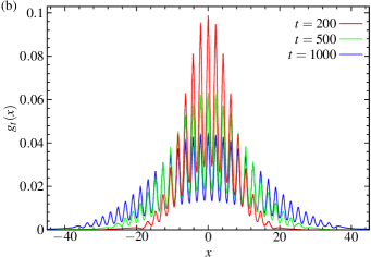
Figure 5: (Color online) (a) Time evolution of displacement distribution functions. (b) Time evolution of displacement densities, calculated by numerically differentiating a cubic spline approximation to distribution functions. $r=2.1$; $b=0.2$. The inset in (a) shows the definition of the set $H(x)$ required later.

The distribution functions are smooth, but have a step-like structure. Differentiating the spline approximations to these distribution functions gives densities which have an underlying gaussian-like shape, modulated by a pronounced fine structure which persists at all times (Fig. 5(b)). This fine structure is just noticeable in Figs. 4 and 5 of Alonso et al. (2002), but otherwise does not seem to have been reported previously, although in the context of iterated 1D maps a fine structure was found, the origin of which is pruning effects: see e.g. Fig. 3.1 of Klages (1996). We will show that in billiards this fine structure can be understood by considering the geometry of the billiard domain.

IV.4 Fine structure of position density

Since Liouville measure on the torus is invariant, if the initial distribution is uniform with respect to Liouville measure, then the distribution at any time $t$ is still uniform. Integrating over the velocities, the position distribution at time $t$ is hence always uniform with respect to Lebesgue measure in the billiard domain $Q$, which we normalize such that the measure of $Q$ is $1$. Denote the two-dimensional position density on the torus at $(x,y)\in[0,1)^{2}$ by $\rho^{\textrm{torus}}(x,y)$. Then

$$\rho^{\textrm{torus}}(x,y)=\frac{1}{\left|Q\right|}\openone_{Q}(x,y)=\frac{1}{\left|Q\right|}\openone_{H(x)}(y).$$ (15)

Here, $H(x):=\{y:(x,y)\in Q\}$ is the set of allowed $y$ values for particles with horizontal coordinate $x$ (Fig. 5(a) inset), and $\openone_{B}$ is the indicator function of the (one- or two-dimensional) set $B$, given by

$$\openone_{B}(b)=\begin{cases}1,\quad\text{if }b\in B\\ 0,\quad\text{otherwise}.\end{cases}$$ (16)

Thus for fixed $x$, $\rho^{\textrm{torus}}(x,y)$ is independent of $y$ within the available space $H(x)$.

Now unfold the dynamics onto a 1-dimensional channel in the $x$-direction, as in Fig. 2, and consider the torus as the distinguished unit cell at the origin. Fix a vertical line with horizontal coordinate $x$ in this cell, and consider its periodic translates $x+n$ along the channel, where $n\in\mathbb{Z}$. Denoting the density there by $\rho^{\textrm{channel}}_{t}(x+n,y)$, we have that for all $t$ and for all $x$ and $y$,

$$\sum_{n\in\mathbb{Z}}\rho^{\textrm{channel}}_{t}(x+n,y)=\rho^{\textrm{torus}}(x,y).$$ (17)

We expect that after a sufficiently long time, the distribution within cell $n$ will look like the distribution on the torus, modulated by a slowly-varying function of $x$. In particular, we expect that the 2D position density will become asymptotically uniform in $y$ within $H(x)$ at long times. We have not been able to prove this, but we have checked by constructing 2D kernel density estimates Silverman (1986) that it seems to be correct. A ‘sufficiently long’ time would be one which is much longer than the time required for the diffusion process to cross one unit cell.

Thus we have approximately

$$\rho^{\textrm{channel}}_{t}(x,y)\simeq\rho^{\textrm{torus}}(x,y)\,\bar{\rho}_{t}(x)=\bar{\rho}_{t}(x)\frac{1}{\left|Q\right|}\openone_{H(x)}(y),$$ (18)

where $\bar{\rho}_{t}(x)$ is the shape of the two-dimensional density distribution as a function of $x\in\mathbb{R}$; we expect this to be a slowly-varying function. We use ‘$\simeq$’ to denote that this relationship holds in the long-time limit, for values of $x$ which do not lie in the tails of the distribution. Although this breaks down in the tails, the density is in any case small there.

The 1D marginal density that we measure will then be given approximately by

$$f_{t}(x)=\int_{y=0}^{1}\rho^{\textrm{channel}}_{t}(x,y)\,\textrm{d}y\simeq\bar{\rho}_{t}(x)\,h(x),$$ (19)

where $h(x):=\left|H(x)\right|/\left|Q\right|$ is the normalized height (Lebesgue measure) of the set $H(x)$ at position $x$ (see the inset of Fig. 5(a)). Note that $H(x)$ is not necessarily a connected set.

Thus the measured density $f_{t}(x)$ is given by the shape $\bar{\rho}_{t}(x)$ of the 2D density, modulated by fine-scale oscillations due to the geometry of the lattice and described by $h(x)$, which we call the fine structure function.

The above argument motivates the (re-)definition of $\bar{\rho}_{t}(x)$ so that that $f_{t}(x)=h(x)\bar{\rho}_{t}(x)$, now with strict equality and for all times. We can then view $\bar{\rho}_{t}(x)$ as the density with respect to a new underlying measure $h\,\lambda$, where $\lambda$ is $1$-dimensional Lebesgue measure; this measure takes into account the available space, and is hence more natural in this problem. We expect that $\bar{\rho}_{t}$ will now describe the large-scale shape of the density, at least for long times and $x$ comparatively small.

Figure 6 shows the original and demodulated densities $f_{t}$ and $\bar{\rho}_{t}$ for a representative choice of geometrical parameters. The fine structure in $f_{t}$ is very pronounced, but is eliminated nearly completely when demodulated by dividing by the fine structure $h$, leaving a demodulated density $\bar{\rho}_{t}$ which is close to the gaussian density with variance $2Dt$ (also shown).

We estimated the diffusion coefficient $D$ as follows. For $r=2.3$ and $b=0.5$, using $N=10^{7}$ particles evolved to $t=1000$, the best fit line for $\log\langle\Delta x^{2}\rangle_{t}$ against $\log t$ in the region $t\in[500,1000]$ gives $\langle\Delta x^{2}\rangle\sim t^{1.00003}$, which we regard as confirmation of asymptotic linear growth. Following Klages and Dellago (2000), we use the slope of $\log\langle\Delta x^{2}\rangle_{t}$ against $t$ in that region as an estimate of $2D$, giving $D=0.1494\pm 0.0002$; see Sanders ; Sanders (2004) for the error analysis.

(Throughout the paper, we denote by $\gamma_{\sigma^{2}}$ the gaussian density with mean $0$ and variance $\sigma^{2}$, and by $N_{\sigma^{2}}$ the corresponding normal distribution function.)

Note that although the density has non-smooth points, which affects the smoothness assumption in our density estimation procedure described in Sec. IV.2, in practice these points are still handled reasonably well. If necessary, we could treat these points more carefully, by suitable choices of partition points in that method.

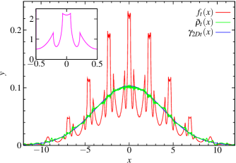
Figure 6: (Color online) Position density $f_{t}$ exhibiting a pronounced fine structure, together with the demodulated slowly-varying function $\bar{\rho}_{t}$ and a gaussian with variance $2Dt$. The inset shows one period of the demodulating fine structure function $h$. $r=2.3$; $b=0.5$; $t=50$.

IV.5 Fine structure of displacement density

We can treat the displacement density similarly, as follows. Let $\eta_{t}(x,y)$ be the 2D displacement density function at time $t$, so that

$$\int_{-\infty}^{x}\int_{\infty}^{y}\eta_{t}(x,y)\,\textrm{d}x\,\textrm{d}y=\mathbb{P}\left(\Delta x_{t}\leq x,\Delta y_{t}\leq y\right),\quad x,y\in\mathbb{R}.$$ (20)

(Recall that $\Delta x_{t}:=x_{t}-x_{0}$.) We define the projected versions $\eta^{\textrm{channel}}$ and $\eta^{\textrm{torus}}$ as follows:

$$\eta^{\textrm{channel}}_{t}(x,y):=\sum_{n\in\mathbb{Z}}\eta_{t}(x,y+n),\quad x\in\mathbb{R},y\in[0,1),$$ (21)

$$\eta^{\textrm{torus}}_{t}(x,y):=\sum_{n\in\mathbb{Z}}\eta^{\textrm{channel}}_{t}(x+n,y),\quad x,y\in[0,1).$$ (22)

Again we view the torus as the unit cell at the origin where all initial conditions are placed. Note that projecting the displacement distribution on $\mathbb{R}^{2}$ to the channel or torus gives the same result as first projecting and then obtaining the displacement distribution in the reduced geometry. Hence the designations as being associated with the channel or torus are appropriate.

Unlike $\rho^{\textrm{torus}}$ in the previous section, $\eta^{\textrm{torus}}_{t}$ is not independent of $t$: for example, for small enough $t$, all displacements increase with time. However, we show that $\eta^{\textrm{torus}}_{t}$ rapidly approaches a distribution which is stationary in time.

Consider a small ball of initial conditions of positive Liouville measure around a point $(\mathbf{x},\mathbf{v})$. Since the system is mixing on the torus, the position distribution at time $t$ corresponding to those initial conditions converges as $t\to\infty$ to a distribution which is uniform with respect to Lebesgue measure in the billiard domain $Q$. The corresponding limiting displacement distribution is hence obtained by averaging the displacement of $\mathbf{x}$ from all points on the torus.

Extending this to an initial distribution which is uniform with respect to Liouville measure over the whole phase space, we see that the limiting displacement distribution is given by averaging displacements of two points in $Q$, with both points distributed uniformly with respect to Lebesgue measure on $Q$. This limiting distribution we denote by $\eta^{\textrm{torus}}(x,y)$, with no $t$ subscript.

As in the previous section, we expect the $y$-dependence of $\eta^{\textrm{channel}}_{t}(x+n,\cdot)$ to be the same, for large enough $t$, as that of $\eta^{\textrm{torus}}(x,\cdot)$ for $x\in[0,1)$. However, $\eta^{\textrm{torus}}(x,\cdot)$ is not independent of $y$, as can be seen from a projected version of Fig. 4(b) on the torus Sanders (2004). We thus set

$$\eta^{\textrm{channel}}_{t}(x,y)\simeq\eta^{\textrm{torus}}(x,y)\,\bar{\eta}_{t}(x).$$ (23)

To obtain the 1D marginal density $g_{t}(x)$, we integrate with respect to $y$:

$$g_{t}(x)=\int_{y=0}^{1}\eta^{\textrm{channel}}_{t}(x,y)\,\textrm{d}y\simeq\phi(x)\bar{\eta}_{t}(x),$$ (24)

where

$$\phi(x):=\int_{y=0}^{1}\eta^{\textrm{torus}}(x,y)\,\textrm{d}y.$$ (25)

Again we now redefine $\bar{\eta}$ so that $g_{t}(x)=\phi(x)\bar{\eta}_{t}(x)$, with the fine structure of $g_{t}(x)$ being described by $\phi$ and the large-scale variation by $\bar{\eta}(x)$, which can be regarded as the density with respect to the new measure $\phi\,\lambda$ taking account of the excluded volume. In the next section we evaluate $\phi(x)$ explicitly.

IV.6 Calculation of $x$-displacement density $\phi(x)$ on torus

Let $(X_{1},Y_{1})$ and $(X_{2},Y_{2})$ be independent random variables, distributed uniformly with respect to Lebesgue measure in the billiard domain $Q$, and let $\Delta X:=\left\{X_{2}-X_{1}\right\}\in[0,1)$ be their $x$-displacement (where $\left\{\cdot\right\}$ again denotes the fractional part of its argument). Then $\Delta X$ is the sum of two independent random variables, so that its density $\phi$ is given by the following convolution, which correctly takes account of the periodicity of $h$ and $\phi$ with period $1$:

$$\phi(\xi)=\int_{0}^{1}h(x)\,h(x+\xi)\,\textrm{d}x.$$ (26)

This form leads us to expand in Fourier series:

$$h(x)=\sum_{k\in\mathbb{Z}}\hat{h}(k)\,\mathrm{e}^{2\pi\mathrm{i}kx}=\hat{h}(0)+2\sum_{k\in\mathbb{N}}\hat{h}(k)\,\cos 2\pi kx,$$ (27)

and similarly for $\phi$, where the Fourier coefficients are defined by

$$\hat{h}(k):=\int_{0}^{1}h(x)\,\mathrm{e}^{-2\pi\mathrm{i}kx}\,\textrm{d}x=\int_{0}^{1}h(x)\,\cos(2\pi kx)\,\textrm{d}x.$$ (28)

The last equality follows from the evenness of $h$, and shows that $\hat{h}(k)=\hat{h}(-k)$, from which the second equality in (27) follows. Fourier transforming (26) then gives

$$\hat{\phi}(k)=\hat{h}(k)\,\hat{h}(-k)=\hat{h}(k)^{2}.$$ (29)

Taking the origin in the center of the disk of radius $b$ (see the inset of Fig. 5), the available space function $h$ is given by

$$h(x)=\frac{1}{\left|Q\right|}\left(1-2\sqrt{b^{2}-x^{2}}-2\sqrt{a^{2}-(\textstyle\frac{1}{2}-x)^{2}}\right)$$ (30)

for $x\in[0,1/2)$, and is even and periodic with period $1$. Here we adopt the convention that $\sqrt{\alpha}=0$ if $\alpha<0$ to avoid writing indicator functions explicitly. The evaluation of the Fourier coefficients of $h$ thus involves integrals of the form

$$\int_{0}^{a}\cos zt\,\sqrt{a^{2}-t^{2}}\,\textrm{d}t=\frac{\pi a}{2z}\,J_{1}(za),\qquad(z\neq 0)$$ (31)

where $J_{1}$ is the first order Bessel function; this equality follows from equation (9.1.20) of Abramowitz and Stegun (1970) after a change of variables.

Hence the Fourier coefficients of $h$ are $\hat{h}(0)=\int_{0}^{1}h(x)=1$ and, for integer $k\neq 0$,

$$\ \hat{h}(k)=-\frac{1}{\left|Q\right|.\left|k\right|}\left[(-1)^{k}\,a\,J_{1}(2\pi a\left|k\right|)+b\,J_{1}(2\pi b\left|k\right|)\right].$$ (32)

Note that $\int_{0}^{1}\phi(x)\,\textrm{d}x=\hat{\phi}(0)=\hat{h}(0)^{2}=1$, so that $\phi$ is correctly normalized as a density function on the torus.

In Fig. 7 we plot partial sums $\phi_{m}$ up to $m$ terms of the Fourier series for $\phi$ analogous to (27). We can determine the degree of smoothness of $\phi$, and hence presumably of $g_{t}$, as follows. The asymptotic expansion of $J_{1}(z)$ for large real $z$ (equation (9.2.1) of Abramowitz and Stegun (1970)),

$$J_{1}(z)\sim\sqrt{\frac{2}{\pi z}}\,\cos\left({\frac{3\pi}{4}}-z\right)=\mathcal{O}(z^{-1/2}),$$ (33)

shows that $\hat{h}(k)=\mathcal{O}(k^{-3/2})$ and hence $\hat{\phi}(k)=\mathcal{O}(k^{-3})$. From the theory of Fourier series (see e.g. (Katznelson, 2004, Chap. 1)), we hence have that $\phi$ is at least $C^{1}$ (once continuously differentiable). Thus the convolution of $h$ with itself is smoother than $h$ is, as intuitively expected, despite the non-differentiable points of $h$.

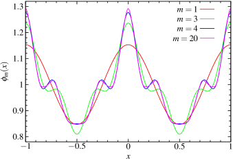
Figure 7: (Color online) Partial sums $\phi_{m}$ up to $m$ terms of the Fourier series for $\phi$, with $r=2.3$ and $b=0.5$.

We have checked numerically the approach of $\int\eta^{\textrm{torus}}_{t}(x,y)\,\textrm{d}y$ to $\phi(x)$, and it appears to be fast, although the rate is difficult to evaluate, since a large number of initial conditions are required for the numerically calculated distribution function to approach closely the limiting distribution.

IV.7 Structure of displacement distribution

In Fig. 8 we plot the numerically-obtained displacement density $g_{t}(x)$, the fine structure function $\phi$ calculated above, and their ratio $\bar{\eta}_{t}(x)$, for a certain choice of geometrical parameters. Again the ratio is approximately gaussian, which confirms that the densities can be regarded as a gaussian shape modulated by the fine structure $\phi$.

However, if $r$ is close to $2a$, then $\bar{\eta}_{t}$ itself develops a type of fine structure: it is nearly constant over each unit cell. This is shown in Fig. 9 for two different times. We plot both $g_{t}$ and $\bar{\eta}_{t}$, rescaled by $\sqrt{t}$ and compared to a gaussian of variance $2D$. (This scaling is discussed in Sec. V.)

This step-like structure of $\bar{\eta}_{t}$ is related to the validity of the Machta–Zwanzig random walk approximation, which gives an estimate of the diffusion coefficient in regimes where the geometrical structure can be regarded as a series of traps with small exits Machta and Zwanzig (1983); Klages and Dellago (2000); Klages and Korabel (2002); Sanders . Having $\bar{\eta}_{t}$ constant across each cell indicates that the distribution of particles within the billiard domain in each cell is uniform, as is needed for the Machta–Zwanzig approximation to work.

As $r$ increases away from $2a$, the exit size of the traps increases, and the Machta–Zwanzig argument ceases to give a good approximation Sanders ; Klages and Dellago (2000). The distribution then ceases to be uniform in each cell: see Fig. 6. This may be related to the crossover to a Boltzmann regime described in Klages and Dellago (2000).

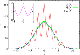
Figure 8: (Color online) Displacement density $g_{t}$, with demodulated $\bar{\eta}_{t}$ compared to a gaussian of variance $2D$. The inset in (a) shows the fine structure function $\phi$ for these geometrical parameters. $r=2.1$; $b=0.2$; $t=50$.

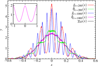
Figure 9: (Color online) Displacement density $g_{t}$ and demodulated $\bar{\eta}_{t}$, both rescaled by $\sqrt{t}$, at $t=200$ and $t=1000$, compared to a gaussian of variance $2D$. The inset again shows the fine structure function $\phi$. $r=2.01$; $b=0.1$.

V Central limit theorem and rate of convergence

We now discuss the central limit theorem as $t\to\infty$ in terms of the fine structure described in the previous section.

V.1 Central limit theorem: weak convergence to normal distribution

The central limit theorem requires us to consider the densities rescaled by $\sqrt{t}$, so we define

$$\tilde{g}_{t}(x):=\sqrt{t}\,g_{t}(x\sqrt{t}),$$ (34)

where the first factor of $\sqrt{t}$ normalizes the integral of $\tilde{g}_{t}$ to $1$, giving a probability density. Figure 10 shows the densities of Fig. 5(a) rescaled in this way, compared to a gaussian density with mean $0$ and variance $2D$. We see that the rescaled densities oscillate within an envelope which remains approximately constant, but with an increasing frequency as $t\to\infty$; they are oscillating around the limiting gaussian, but do not converge to it pointwise. See also Fig. 9.

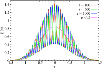
Figure 10: (Color online) Displacement densities as in Fig. 5(b) after rescaling by $\sqrt{t}$, compared to a gaussian density with mean $0$ and variance $2D$. $r=2.1$; $b=0.2$.

The increasingly rapid oscillations do, however, cancel out when we consider the rescaled distribution functions, given by the integral of the rescaled density functions:

$$\tilde{G}_{t}(x):=\int_{s=-\infty}^{x}\tilde{g}_{t}(s)\,\textrm{d}s=G_{t}(x\,\sqrt{t}).$$ (35)

Figure 11 shows the difference between the rescaled distribution functions and the limiting normal distribution with mean $0$ and variance $2D$. We see that the rescaled distribution functions do converge to the limiting normal, in fact uniformly, as $t\to\infty$; we thus have weak convergence.

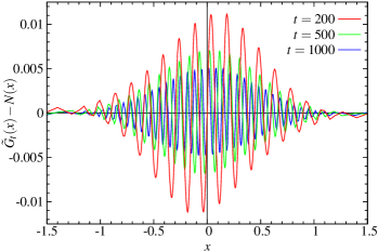
Figure 11: (Color online) Difference between rescaled distribution functions and limiting normal distribution with variance $2D$. $r=2.1$; $b=0.2$.

Although this is the strongest kind of convergence we can obtain for the densities $\tilde{g}_{t}$ with respect to Lebesgue measure, Fig. 9 provides evidence for the following conjecture: the rescaled densities $\tilde{\bar{\eta}}_{t}$ with respect to the new, modulated measure converge uniformly to a gaussian density. This characterizes the asymptotic behavior more precisely than the standard central limit theorem.

V.2 Rate of convergence

Since the $\tilde{G}_{t}$ converge uniformly to the limiting normal distribution, we can consider the distance $\left\|\tilde{G}_{t}-N_{2D}\right\|_{\infty}$, where we define the uniform norm by

$$\left\|F\right\|_{\infty}:=\sup_{x\in\mathbb{R}}\left|F(x)\right|.$$ (36)

We denote by $N_{\sigma^{2}}$ the normal distribution function with variance $\sigma^{2}$, given by

$$N_{\sigma^{2}}(x):=\frac{1}{\sigma\sqrt{2\pi}}\int_{s=-\infty}^{x}\mathrm{e}^{-s^{2}/2\sigma^{2}}\,\textrm{d}s,$$ (37)

Figure 12 shows a log–log plot of this distance against time, calculated numerically from the full distribution functions. We see that the convergence follows a power law

$$\left\|\tilde{G}_{t}-N_{2D}\right\|_{\infty}\sim t^{-\alpha},$$ (38)

with a fit to the data for $r=2.05$ giving a slope $\alpha\simeq 0.482$. The same decay rate is obtained for a range of other geometrical parameters, although the quality of the data deteriorates for larger $r$, reflecting the fact that diffusion is faster, so that the distribution spreads further in the same time. Since we use the same number $N=10^{7}$ of initial conditions, there is a lower resolution near $x=0$ where, as shown in the next section, the maximum is obtained.

In Pène (2002) it was proved rigorously that $\alpha\geq\frac{1}{6}\simeq 0.167$ for any Hölder continuous observable $f$. Here we have considered only the particular Hölder observable $v$, but for this function we see that the rate of convergence is much faster than the lower bound proved in Pène (2002).

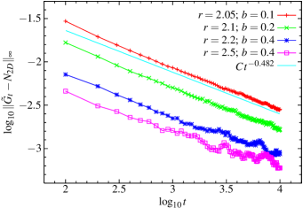
Figure 12: (Color online) Distance of rescaled distribution functions $\tilde{G}_{t}$ from limiting normal distribution $N_{2D}$ in log–log plot. The straight line is a fit to the large-time decay of the data for $r=2.05$.

V.3 Analytical estimate of rate of convergence

We now obtain a simple analytical estimate of the rate of convergence using the fine structure calculations in Sec. IV.

Since the displacement distribution is symmetric, we have $\tilde{G}_{t}(x=0)=1/2$ for all $t$. The maximum deviation of $\tilde{G}_{t}$ from $N_{2D}$ occurs near to $x=0$, where the density function is furthest from a gaussian, while the fine structure of the density $\tilde{g}_{t}$ means that $\tilde{G}_{t}$ is increasing there (Fig. 11). Due to the oscillatory nature of the fine structure, this maximum thus occurs at a distance of $1/4$ of the period of oscillation from $x=0$.

Since the displacement density has the form $g_{t}(x)=\phi(x)\bar{\eta}_{t}(x)$, after rescaling we have

$$\tilde{g}_{t}(x)=\phi(x\sqrt{t})\tilde{\bar{\eta}}(x),$$ (39)

where $\tilde{\bar{\eta}}_{t}(x):=\sqrt{t}\,\bar{\eta}_{t}(x\sqrt{t})$ is the rescaled slowly-varying part of $g_{t}$, and the fine structure at time $t$ is given by

$$\phi(x\sqrt{t})=1+2\sum_{k\in\mathbb{N}}\hat{\phi}(k)\,\cos(2\pi kx\sqrt{t}).$$ (40)

The maximum deviation occurs at $1/4$ of the period of $\phi(x\sqrt{t})$, i.e. at $x=\frac{1}{4\sqrt{t}}$, so that

$$\left\|G_{t}-N\right\|_{\infty} \simeq\int_{0}^{1/4\sqrt{t}}\sum_{k\in\mathbb{N}}\hat{\phi}(k)\,\cos(2\pi kx\sqrt{t})\,\textrm{d}x$$ (41)

$$=\frac{1}{\sqrt{t}}\sum_{k\in\mathbb{N},\,k\text{ odd}}\hat{\phi}(k)\frac{(-1)^{(k-1)/2}}{2\pi k}.$$ (42)

The correction due to the curvature of the underlying gaussian converges to $0$ as $t\to\infty$, since this gaussian is flat at $x=0$. Hence $\left\|G_{t}-N\right\|_{\infty}=\mathcal{O}(t^{-1/2})$.

This calculation shows that the fastest possible convergence is a power law with exponent $\alpha=1/2$, and provides an intuitive reason why this is the case. If the rescaled shape function $\tilde{\bar{\eta}}_{t}$ converges to a gaussian shape at a rate slower than $t^{-1/2}$, then the overall rate of convergence $\alpha$ could be slower than $1/2$. However, the numerical results in Sec. V.2 show that the rate is close to $1/2$. We remark that for an observable which is not so intimately related to the geometrical structure of the lattice, the fine structure will in general be more complicated, and the above argument may no longer hold.

VI Maxwellian velocity distribution

In this section we consider the effect of a non-constant distribution of particle speeds . A Maxwellian (gaussian) velocity distribution was used in polygonal and Lorentz channels in Li et al. (2003) and Alonso et al. (1999), respectively, in connection with heat conduction studies. The mean square displacement was observed to grow asymptotically linearly, but the relationship with the unit speed situation was not discussed. A more complicated Lorentz gas with a gaussian distribution was studied in Klages et al. (2000).

We show that the mean square displacement grows asymptotically linearly in time with the same diffusion coefficient as for the unit speed case, but that the limiting position distribution may be non-gaussian. For brevity we refer only to the position distribution throughout this section; the displacement distribution is similar.

VI.1 Mean square displacement

Consider a particle located initially at $(\mathbf{x}_{0},\mathbf{v}_{0})$, where $\mathbf{v}_{0}$ has unit speed. Changing the speed of the particle does not change the path it follows, but only the distance along the path traveled in a given time. Denoting by $\Phi_{v}^{t}(\mathbf{x}_{0},\mathbf{v}_{0})$ the billiard flow with speed $v$ starting from $\mathbf{x}_{0}$ and with initial velocity in the direction of the unit vector $\mathbf{v}_{0}$, we have

$$\Phi_{v}^{t}(\mathbf{x}_{0},\mathbf{v}_{0})=\Phi^{vt}(\mathbf{x}_{0},\mathbf{v}_{0}),$$ (43)

where the flow on the right hand side is the original unit-speed flow. If all speeds are equal to $v$, then the radially symmetric 2D position probability density after a long time $t$ is thus

$$p_{t}\left(x,y\,\big{|}\,v\right)=\frac{1}{4\pi Dvt}\exp\left(\frac{-(x^{2}+y^{2})}{4Dvt}\right),$$ (44)

giving a radial density

$$p_{t}\left(r\,\big{|}\,v\right)=\frac{r}{2Dvt}\,\exp\left(\frac{-r^{2}}{4Dvt}\right).$$ (45)

(Throughout this calculation we neglect any fine structure.)

If we now have a distribution of velocities with density $p_{V}(v)$, then the radial position density at distance $r$ is

$$f^{\text{rad}}_{t}(r)=\int_{v=0}^{\infty}p_{t}\left(r\,\big{|}\,v\right)\,p_{V}(v)\,\textrm{d}v.$$ (46)

The variance of the position distribution is then given by

$$\langle\mathbf{x}^{2}\rangle =\int_{r=0}^{\infty}r^{2}\,f^{\text{rad}}_{t}(r)\,\textrm{d}r$$ (47)

$$=4Dt\int_{0}^{\infty}v\,p_{V}(v)\,\textrm{d}v=:4Dt\bar{v},$$ (48)

where $\bar{v}$ is the mean speed, after interchanging the integrals over $r$ and $v$.

We thus see that for any speed distribution having a finite mean, the variance of the position distribution, and hence the mean square displacement, grows asymptotically linearly with the same diffusion coefficient as for the uniform speed distribution, having normalized such that $\bar{v}=1$. We have verified this numerically with a gaussian velocity distribution: the mean square displacement is indistinguishable from the unit speed case even after very short times Sanders (2004).

VI.2 Gaussian velocity distribution

Henceforth attention is restricted to the case of a gaussian velocity distribution. For each initial condition, we generate two independent normally-distributed random variables $v_{1}$ and $v_{2}$ with mean $0$ and variance $1$ using the standard Box–Muller algorithm Press et al. (1992), and then multiply by $\sigma$, which is a standard deviation calculated below. We use $v_{1}$ and $v_{2}$ as the components of the velocity vector $\mathbf{v}$, whose probability density is hence given by

$$p(\mathbf{v})=p(v_{1},v_{2})=\frac{\mathrm{e}^{-v_{1}^{2}/2\sigma^{2}}}{\sigma\sqrt{2\pi}}\,\,\frac{\mathrm{e}^{-v_{2}^{2}/2\sigma^{2}}}{\sigma\sqrt{2\pi}}\,=\frac{\mathrm{e}^{-v^{2}/2\sigma^{2}}}{2\pi\sigma^{2}}\,,$$ (49)

where $v:=\left|\mathbf{v}\right|=\sqrt{v_{1}^{2}+v_{2}^{2}}$ is the speed of the particle. The speed $v$ thus has density

$$p_{V}(v)=\frac{v}{\sigma^{2}}\,\mathrm{e}^{-v^{2}/2\sigma^{2}}$$ (50)

and mean $\bar{v}=\sigma\sqrt{\pi/2}$. To compare with the unit speed distribution we require $\bar{v}=1$, and hence $\sigma=\sqrt{2/\pi}$. As before, we distribute the initial positions uniformly with respect to Lebesgue measure in the billiard domain $Q$.

VI.3 Shape of limiting distribution

The position density (46) is a function of time. However, the gaussian assumption used to derive that equation is valid in the limit when $t\to\infty$, so the central limit theorem rescaling

$$\tilde{f}^{\text{rad}}_{t}(r):=\sqrt{t}\,f^{\text{rad}}_{t}(r\sqrt{t})$$ (51)

eliminates the time dependence in (46), giving the following shape for the limiting radial density:

$$\tilde{f}^{\text{rad}}(r)=\frac{\pi r}{4D}\int_{v=0}^{\infty}\exp\left(-\frac{r^{2}}{4Dv}-\frac{\pi v^{2}}{4}\right)\,\textrm{d}v=:\frac{\pi r}{4D}\,I,$$ (52)

denoting the integral by $I$. Mathematica Wolfram (2004) can evaluate this integral explicitly in terms of the Meijer $G$-function Erdélyi et al. (1953):

$$I=G^{3,0}_{0,3}\left(\frac{\pi r^{4}}{256D^{2}}\right|\left.\begin{matrix}\text{---}\\ -\textstyle\frac{1}{2},0,0\end{matrix}\right).$$ (53)

See Metzler and Klafter (2000) and references therein for a review of the use of such special functions in anomalous diffusion.

We can, however, obtain an asymptotic approximation to $I$ from its definition as an integral, without using any properties of special functions, as follows. Define $K(v):=\frac{r^{2}}{4Dv}+\frac{\pi v^{2}}{4}$, the negative of the argument of the exponential in (52). Then $K$ has a unique minimum at $v_{\text{min}}:=(r^{2}/(2\pi D))^{1/3}$ and we expect the integral to be dominated by the neighborhood of this minimum. However, the use of standard asymptotic methods is complicated by the fact that as $r\to 0$, $v_{\text{min}}$ tends to $0$, a boundary of the integration domain.

To overcome this, we change variables to fix the minimum away from the domain boundaries, setting $w:=v/v_{\text{min}}$. Then

$$I=v_{\text{min}}\int_{w=0}^{\infty}e^{-\alpha\,L(w)}\,\textrm{d}w,$$ (54)

where $\alpha:=\frac{\pi v_{\text{min}}^{2}}{2}$ and $L(w):=\frac{1}{w}+\frac{w^{2}}{2}$, with a minimum at $w_{\text{min}}=1$. Laplace’s method (see e.g. Carrier et al. (1966)) can now be applied, giving the asymptotic approximation

$$I\sim v_{\text{min}}\,e^{-\alpha L(w_{\text{min}})}\frac{\sqrt{2\pi}}{\sqrt{\alpha\,L^{\prime\prime}(w_{\text{min}})}}=\frac{2}{\sqrt{3}}e^{-3\alpha/2},$$ (55)

valid for large $\alpha$, i.e. for large $r$.

Hence

$$\tilde{f}^{\text{rad}}(r)\stackrel{{\scriptstyle r\to\infty}}{{\sim}}C\,r\,e^{-\beta\,r^{4/3}},$$ (56)

where

$$C:=\frac{\pi}{2D\sqrt{3}};\quad\beta:=\frac{3}{2}\left(\frac{\pi}{32D^{2}}\right)^{1/3}.$$ (57)

VI.4 Comparison with numerical results

Figure 13 shows the numerical radial position density $\tilde{f}^{\text{rad}}_{t}(r)$ for a particular choice of geometrical parameters. We wish to demodulate this as in Sec. IV to extract the slowly-varying shape function, which we can then compare to the analytical calculation.

The radial fine structure function $\phi^{\text{rad}}(r)$ must be calculated numerically, since no analytical expression is available. We do this by distributing $10^{5}$ points uniformly on a circle of radius $r$ and calculating the proportion of points not falling inside any scatterer. This we normalize so that $\phi^{\text{rad}}(r)\to 1$ as $r\to\infty$, using the fact that when $r$ is large, the density inside the circle of radius $r$ converges to the ratio $[r^{2}-\pi(a^{2}+b^{2})]/r^{2}$ of available area per unit cell to total area per unit cell. We can then demodulate $\tilde{f}^{\text{rad}}_{t}$ by $\phi^{\text{rad}}$, setting

$$\tilde{\rho}^{\text{rad}}_{t}(r):=\frac{\tilde{f}^{\text{rad}}_{t}(r)}{\phi^{\text{rad}}(r\,\sqrt{t})}.$$ (58)

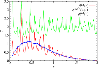
Figure 13: (Color online) The radial density function $\tilde{f}^{\text{rad}}_{t}$ compared to the numerically calculated radial fine structure function $\phi^{\text{rad}}$, rescaled to converge to $1$ and then vertically shifted for clarity. The demodulated radial density $\tilde{\rho}^{\text{rad}}_{t}$ is also shown. $r=2.3$; $b=0.5$; $t=100$.

Figure 13 shows the demodulated radial density $\tilde{\rho}^{\text{rad}}_{t}(r)$ at two times compared to the exact solution (52)–(53), the asymptotic approximation (56)–(57), and the radial gaussian $\frac{r}{2D}e^{-r^{2}/2D}$. The asymptotic approximation agrees well with the exact solution except at the peak, while the numerically determined demodulated densities agree with the exact long-time solution over the whole range of $r$. All three differ significantly from the gaussian, even in the tails. We conclude that the radial position distribution is non-gaussian. A similar calculation could be done for the radial displacement distribution, but a numerical integration would be required to evaluate the relevant fine structure function.

An explanation of the non-gaussian shape comes by considering slow particles which remain close to the origin for a long time, and fast particles which can travel further than those with unit speed. The combined effect skews the resulting distribution in a way which depends on the relative weights of slow and fast particles.

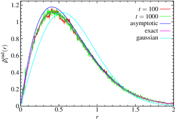
Figure 14: (Color online) Comparison of the demodulated radial density $\tilde{\rho}^{\text{rad}}_{t}$ with the exact Meijer-$G$ representation, the large-$r$ asymptotic approximation, and the radial gaussian with variance $2D$.

VI.5 1D marginal

The 1D marginal in the $x$-direction is shown in Fig. 15. Again there is a significant deviation of the demodulated density from a gaussian. From (56), the 2D density at $(x,y)$ is asymptotically

$$\tilde{f}(x,y)\sim\frac{C}{2\pi}\exp\left[-\beta(x^{2}+y^{2})^{2/3}\right],$$ (59)

from which the 1D marginal $\tilde{f}(x)$ is obtained by

$$\tilde{f}(x)=\int_{y=-\infty}^{\infty}\tilde{f}(x,y)\,\textrm{d}y.$$ (60)

It does not seem to be possible to perform this integration explicitly for either the asymptotic expression (59) or the corresponding exact solution in terms of the Meijer $G$-function. Instead we perform another asymptotic approximation starting, from the asymptotic expression (59). Changing variables in (60) to $z:=y/x$ and using the evenness in $y$ gives

$$\tilde{f}(x)\sim\frac{C\left|x\right|}{2\pi}\int_{z=-\infty}^{\infty}\exp\left[-\kappa(1+z^{2})^{2/3}\right]\,\textrm{d}z,$$ (61)

where $\kappa:=\beta\left|x\right|^{4/3}$. Laplace’s method then gives

$$\tilde{f}(x)\sim\frac{C\sqrt{3}}{\sqrt{8\pi\beta}}\left|x\right|^{1/3}e^{-\beta\left|x\right|^{4/3}},$$ (62)

valid for large $x$. This is also shown in Fig. 15. Due to the $\left|x\right|^{1/3}$ factor, the behavior near $x=0$ is wrong, but in the tails there is reasonably good agreement with the numerical results.

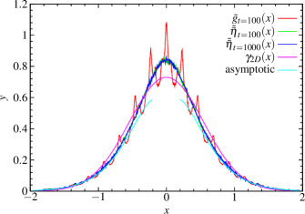
Figure 15: (Color online) Rescaled 1D marginal of the displacement density $\tilde{g}$ and the demodulated version $\tilde{\bar{\eta}}$ compared to the gaussian with variance $2D$ and to the asymptotic expression. The latter is not shown close to $x=0$, where it drops to $0$. $r=2.3$; $b=0.5$.

VII Polygonal billiard channel

In this section, we apply the previous ideas to a polygonal billiard channel. Polygonal models differ from Lorentz gases in that they are not chaotic in the standard sense, since the Kolmogorov–Sinai entropy and all Lyapunov exponents are zero due to the weak nature of the scattering from the polygonal sides van Beijeren (2004). Other indicators of the complexity of the dynamics of such systems are required: see e.g. van Beijeren (2004) and references therein for a recent example.

As far as we aware, there are few rigorous results on ergodic and statistical properties of these models Alonso et al. (2002); Casati and Prosen (1999). However, certain polygonal channels have been found numerically to show normal diffusion, in the sense that our property (a) is satisfied, i.e. the mean squared displacement grows asymptotically linearly: see e.g. Li et al. (2003); Alonso et al. (2002). No convincing evidence has so far been given, however, that property (b), the central limit theorem, can be satisfied, although it was shown in Dettmann and Cohen (2000) that (c) is satisfied for some random polygonal billiard models. Here we show that polygonal billiards can satisfy the central limit theorem.

VII.1 Polygonal billiard channel model

We study a polygonal billiard introduced in Alonso et al. (2002). The geometry is shown in Fig. 16 and the channel in Fig. 16. We fix the angles $\phi_{1}$ and $\phi_{2}$ and choose $d$ such that the width of the bottom triangles is half that of the top triangle. This determines the ratio of $h_{1}$ to $h_{2}$ in terms of the angles $\phi_{1}$ and $\phi_{2}$. We then require the inward-pointing vertices of each triangle to lie on the same horizontal line in order to prevent infinite horizon trajectories, giving $h_{1}+h_{2}=h=1$ and $d=h/(\tan\phi_{1}+\textstyle\frac{1}{2}\tan\phi_{2})$, with $h_{1}=d\tan\phi_{1}$ and $h_{2}=(d/2)\tan\phi_{2}$. We remark that in Alonso et al. (2002) it was stated that the area $\left|Q\right|=dh$ of the billiard domain is independent of $\phi_{2}$ when $\phi_{1}$ is fixed, but this is not correct, since the expression for $d$ shows that it depends on $\phi_{2}$, and we have fixed $h=1$.

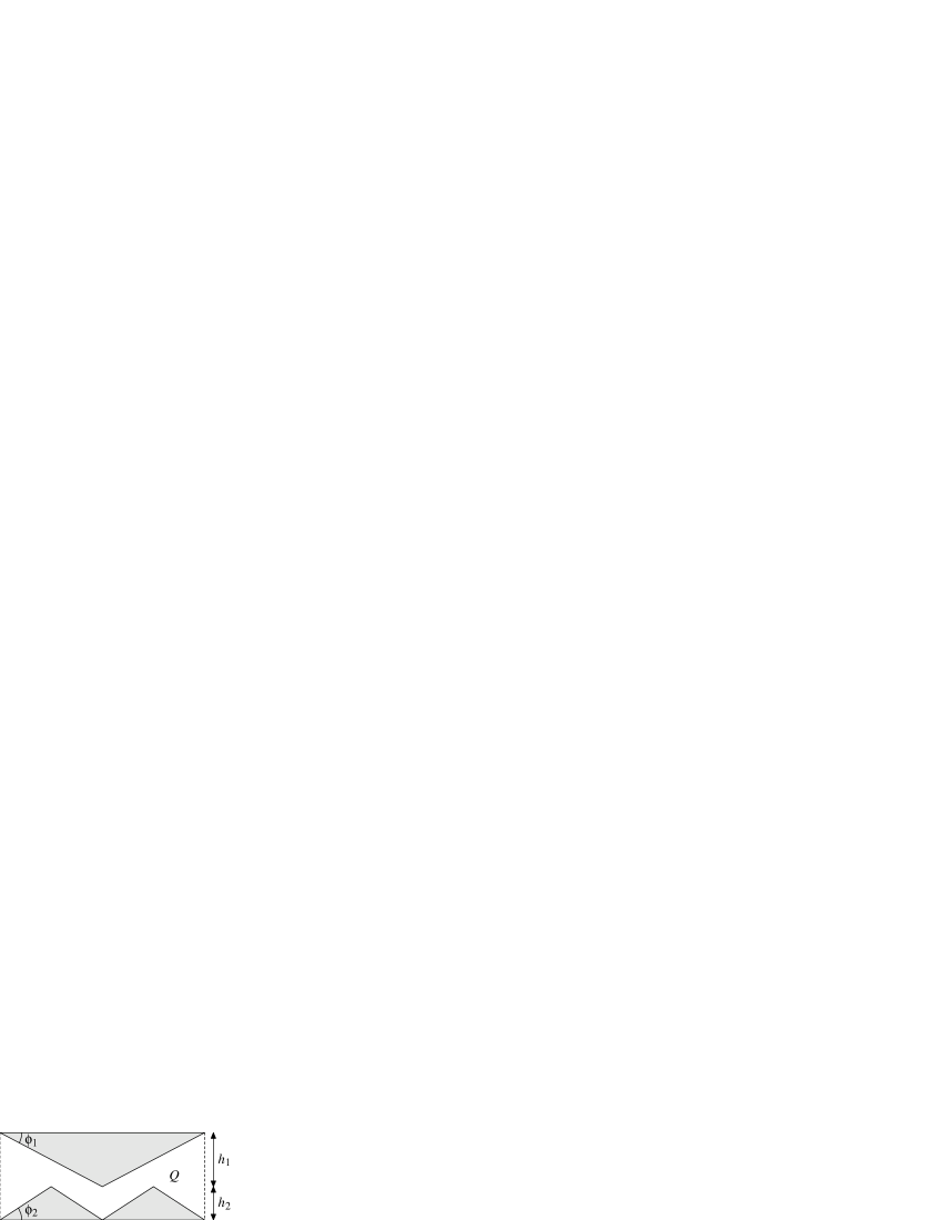
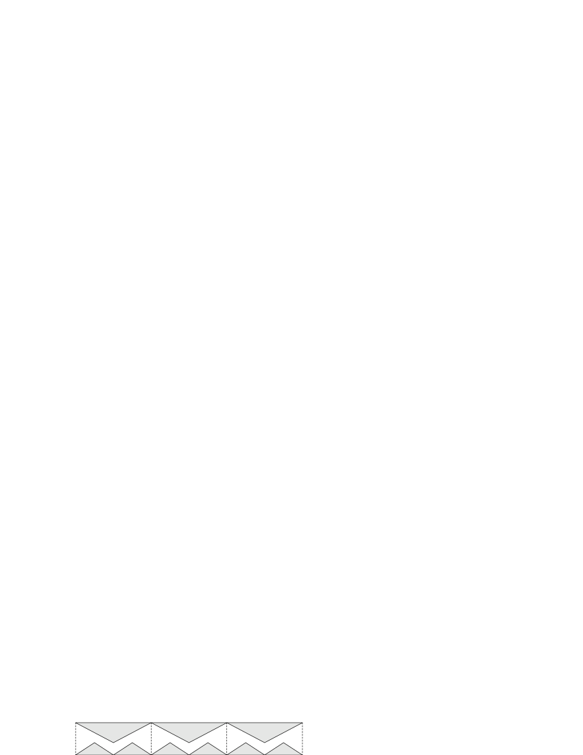
Figure 16: (a) The geometry of the polygonal billiard unit cell, shown to scale with $\phi_{2}=\pi/(2e)$. (b) Part of the polygonal channel with the same parameters.

In Alonso et al. (2002) the parameters $\phi_{1}=\pi(\sqrt{5}-1)/8$ and $\phi_{2}=\pi/q$ were used, with $q\in\mathbb{N}$ and $3\leq q\leq 9$. For $q\geq 5$ normal diffusion was found, whereas for $q=3,4$ it was found that $\langle\Delta x^{2}\rangle_{t}\sim t^{\alpha}$ with $\alpha\neq 1$, so that property (a) is no longer satisfied and we have anomalous diffusion. As far as we are aware, there is as yet no physical or geometrical explanation for this observed anomalous behavior, although presumably number-theoretic properties of the angles are relevant.

We use the same $\phi_{1}$, but a value of $\phi_{2}$ which is irrationally related to $\pi$, namely $\phi_{2}=\pi/(2e)\simeq\pi/5.44$ (where $e$ is the base of natural logarithms), since there is evidence that mixing properties are stronger for such irrational polygons Casati and Prosen (1999). In this case we find $\langle\Delta x^{2}\rangle_{t}\sim t^{1.008}$, which we regard as asymptotically linear, so that property (a) is again satisfied, with $D=0.3796\pm 0.0009$.

VII.2 Fine structure

The shape of the displacement density was considered in Alonso et al. (2002) using histograms, but the results were not conclusive. Here we use our more refined methods to study the fine structure of position and displacement distributions and to show their asymptotic normality.

Figure 17 shows a representative position density $f_{t}(x)$. Following the method of Sec. IV.4, we calculate the fine structure function $h(x)$ as the normalized height of available space at position $x$; this is shown in the inset. We demodulate $f_{t}$ by dividing by $h$ to yield $\bar{\rho}_{t}$, which is again close to the gaussian with variance $2Dt$.

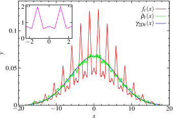
Figure 17: (Color online) Position density at $t=50$ in the polygonal model with $\phi_{2}=\pi/(2e)$. The inset shows $h(x)$ over two periods.

With the same notation as in Sec. IV.6, we can also calculate the fine structure function $\phi$ of the displacement density. Taking the origin in the center of the unit cell in Fig. 16, we have

$$h(x)=\frac{2d}{\left|Q\right|}\left(x\,\tan\phi_{1}+\left|x-\textstyle\frac{1}{2}d\right|\,\tan\phi_{2}\right)$$ (63)

for $0\leq x\leq d$, with $h$ being an even function and having period $2d$. (The factor of $2d$ in (63) makes $h$ a density per unit length.) The Fourier coefficients are $\hat{h}(0)=1$ and

$$\hat{h}(k)=\frac{1}{2d}\int_{-d}^{d}h(x)\,\cos\left(\frac{\pi\,k\,x}{d}\right)=\frac{1}{\left|Q\right|}\frac{d^{2}}{\pi^{2}k^{2}}\,l(k)$$ (64)

for $k\neq 0$, where for $m\in\mathbb{Z}$ we have

$$l(k)=\begin{cases}4\tan(\phi_{1}),&\text{if $k$ odd}\\ 8\tan(\phi_{2}),&\text{if }k=4m+2\\ 0,&\text{if }k=4m.\end{cases}$$ (65)

VII.3 Central limit theorem

As for the Lorentz gas, we rescale the densities and distribution functions by $\sqrt{t}$ to study the convergence to a possible limiting distribution. Again we find oscillation on a finer and finer scale and weak convergence to a normal distribution: see Fig. 18. Figure 19 shows the time evolution of the demodulated densities $\tilde{\bar{\eta}}_{t}$. There is an unexpected peak in the densities near $x=0$ for small times, indicating some kind of trapping effect; this appears to relax in the long time limit. Again we conjecture that we have uniform convergence of the demodulated densities $\tilde{\bar{\eta}}$ to a gaussian density.

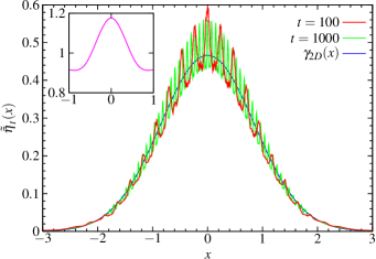
Figure 18: (Color online) Rescaled displacement denstities compared to the gaussian with variance $2D$. The inset shows the function $\phi$ for this geometry.

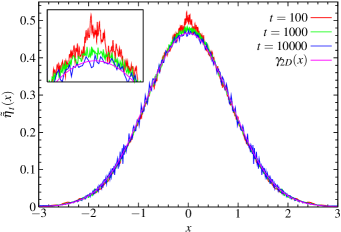
Figure 19: (Color online) Demodulated densities $\tilde{\bar{\eta}}_{t}$ for $t=100$, $t=1000$ and $t=10000$, compared to a gaussian with variance $2D$. The inset shows a detailed view of the peak near $x=0$.

Figure 20 shows the distance of the rescaled distribution functions from the limiting normal distribution, analogously to Fig. 12, for several values of $\phi_{2}$ for which the mean square displacement is asymptotically linear. The straight line fitted to the graph for $\phi_{2}=\pi/(2e)$ has slope $-0.212$, so that the rate of convergence for this polygonal model is substantially slower than that for the Lorentz gas, presumably due to the slower rate of mixing in this system. A similar rate of decay is found for $\phi_{2}=\pi/7$, whilst $\phi_{2}=\pi/6$ and $\phi_{2}=\pi/9$ appear to have a slower decay rate. Nonetheless, the distance does appear to converge to $0$ for all these values of $\phi_{2}$, providing evidence that the distributions are asymptotically normal, i.e. that the central limit theorem is satisfied.

We remark that these convergence rate considerations will be affected if we have not reached the asymptotic regime, which would lead to an incorrect determination of the relevant limiting growth exponent and/or diffusion coefficient.

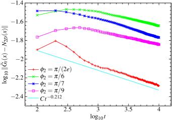
Figure 20: (Color online) Distance of the rescaled distribution functions from the limiting normal distribution for the polygonal model with different values of $\phi_{2}$. The straight line is a fit to the large-time decay of the irrational case $\phi_{2}=\pi/(2e)$.

VIII Conclusions

We have studied deterministic diffusion in diffusive billiards in terms of the central limit theorem. In a 2D periodic Lorentz gas model, where the central limit theorem is proved, we have shown that it is possible to understand analytically the fine structure occurring in the finite-time marginal position and displacement distribution functions, in terms of the geometry of a unit cell. Demodulating the observed densities by the fine structure allowed us to obtain information about the large-scale shape of the densities which would remain obscured without this demodulation: we showed that the demodulated densities are close to gaussian.

We then studied the manner and rate of convergence to the limiting normal distribution required by the central limit theorem. We were able to obtain a simple estimate of the rate of convergence in terms of the fine structure of the distribution functions. The demodulated densities appear to converge uniformly to gaussian densities, which is a strengthening of the usual central limit theorem.

We showed that imposing a Maxwellian velocity distribution does not change the growth of the mean square displacement, but alters the shape of the limiting position distribution to a non-gaussian one.

Finally we showed that similar methods can be applied to a polygonal billiard channel where few rigorous results are available, showing that the central limit theorem can be satisfied by such models, but finding a slower rate of convergence than for the Lorentz gas.

We believe that our analysis may have implications for the escape rate formalism for calculating transport coefficients (see e.g. Gaspard (1998)), where the diffusion equation with absorbing boundary conditions is used as a phenomenological model of the escape process from a finite length piece of a Lorentz gas: analyzing the fine structure in this situation could provide information about the validity of this use of the diffusion equation. We also intend to investigate models exhibiting anomalous diffusion using the methods presented in this paper.