Some incidence theorems and integrable discrete equations V.E. Adler

Institut für Mathematik, Technische Universität Berlin,
Str. des 17. Juni 136, 10623 Berlin, Germany
E-mail: adler@itp.ac.ru

Abstract. Several incidence theorems of planar projective geometry are considered. It is demonstrated that generalizations of Pascal theorem due to Möbius give rise to double cross-ratio equation and Hietarinta equation. The construction corresponding to the double cross-ratio equation is a reduction to a conic section of some planar configuration $(20_{3}15_{4})$. This configuration provides a correct definition of the multidimensional quadrilateral lattices on the plane.

1 Introduction

Accordingly to [1, 8], a $m$-dimensional partial difference equation $F[x]=0$, $x:\mathbb{Z}^{m}\to\mathbb{R}^{d}$, is called integrable if it can be self-consistently imposed on each $m$-dimensional sublattice in $\mathbb{Z}^{m+1}$. Assume that this equation can be interpreted as a geometric construction which defines some elements of a figure by the other ones. This may be a figure not necessarily in $\mathbb{R}^{d}$, for example, $x$ may play the role of parameter on some manifold. Then the integrability means that some complex figure exists which contains several copies of our basic figure, and this complex figure can be constructed by the given elements in several ways. In other words, the self-consistency property is expressed geometrically as some incidence theorem.

In some examples, the construction of the basic figure is itself possible due to an incidence, so that already the equation $F[x]=0$ is equivalent to some incidence theorem. This low-level incidence occurs, when our equation is a reduction in some more general equation, or, geometrically, our construction is a particular case of some more general construction.

The present paper illustrates these notions by the examples of double cross-ratio equation (Nimmo and Schief [9]), Hietarinta equation [4], and quadrilateral lattices (Doliwa and Santini [3]). Recall that double cross-ratio, or discrete Schwarz-BKP equation appears in the theory of Bäcklund transformations for 2+1-dimensional sine-Gordon and Nizhnik-Veselov-Novikov equations and is equivalent to Hirota-Miwa equation and star-triangle map. Its applications in geometry were found in [5, 6]. Quadrilateral lattices can be considered as the discrete analog of the conjugated nets [3] and are the object of intensive study in the modern theory of integrable systems and discrete geometry (see, for example, the recent review [2]).

We start in Section 2 from the Möbius theorem on the polygons inscribed in a conic section and Theorem 2 which is its modification. Section 3 is devoted to the analytical description of the figures under consideration. In Sections 4, 6 we consider in more details the particular cases of these theorems, corresponding to double cross-ratio and Hietarinta equations.

In Section 5 we show that double cross-ratio equation is a reduction of some more general mapping which corresponds geometrically to some planar configuration with the symbol $(20_{3}15_{4})$. In turn, this configuration is just the projection on the plane of the elementary cell of the quadrilateral lattice. Integrability of quadrilateral lattices in $\mathbb{R}^{3}$, proved in [3], implies the integrability of this mapping on the plane, and next, reduction to the conic section proves the integrability of double cross-ratio equation.

In brief, the content of the paper is illustrated by the following diagram.

Möbius theorem  $\stackrel{{\scriptstyle N=3}}{{\longrightarrow}}$  Pascal theorem  $\stackrel{{\scriptstyle N=3}}{{\longleftarrow}}$ Theorem 2     $\big{\downarrow}$ $N=4$     $\big{\downarrow}$ $N=4$ double cross-ratio eq. (10) Hietarinta eq. (14)     $\big{\uparrow}$ reduction to the conic section Theorem 4, quadrilateral lattices on the plane     $\big{\uparrow}$ projection quadrilateral lattices in $\mathbb{R}^{d}$

2 Generalizations of Pascal theorem

Recall that, accordingly to Pascal theorem (the prolongations of) the opposite sides of a hexagon inscribed in a conic section meet on a straight line. In 1847, Möbius found the following generalizations of this theorem (see fig. 1):

1) let $(4n+2)$-gon be inscribed in a conic section and $2n$ pairs of its opposite sides meet on a straight line, then the same is true for the remaining pair;

2) let two $2n$-gons be inscribed in a conic section and $2n-1$ pairs of their corresponding sides meet on a straight line, then the same is true for the remaining pair.

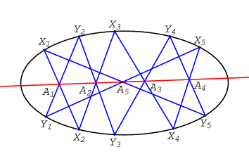
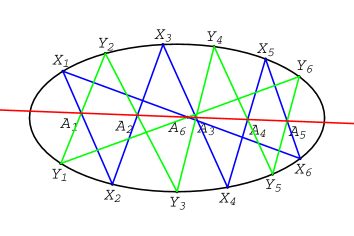
Figure 1: Möbius theorem, $N=5,6$

In order to fix the notations, we reformulate this as follows.

Theorem 1 (Möbius).

Let $X_{1},Y_{1},\dots,X_{N},Y_{N}$ be points on a conic section. Consider the intersection points $A_{j}=X_{j}X_{j+1}\cap Y_{j}Y_{j+1}$, $j=1,\dots N-1$ and

$$A_{N}=\left\{\begin{array}[]{lll}X_{N}Y_{1}\cap Y_{N}X_{1}&\mbox{\rm if}&N=2n+1,\\ X_{N}X_{1}\cap Y_{N}Y_{1}&\mbox{\rm if}&N=2n.\end{array}\right.$$

If all of these points except possibly one are collinear then the same is true for the remaining point.

The proof by Möbius (based on the Gergonne proof of Pascal theorem) is very simple. Consider the projective transformation of the plane which maps the conic section into a circle and sends the line of intersections to infinity. Then the statement is that if all pairs of the opposite (resp. corresponding) sides except for possibly one are parallel then this is true for the remaining pair as well. This easily follows from the fact that a pair of parallel chords cuts off equal arcs of the circle with opposite orientation and vice versa: $XX^{\prime}\;\|\;YY^{\prime}\ \Leftrightarrow\ \widehat{XY}=-\widehat{X^{\prime}Y^{\prime}}$. The change of orientation explains the difference between the cases of odd and even $N$. (Possibly, this was the first step on the way to the invention of the Möbius band, in 1861?)

Another proof can be obtained by applying Pascal theorem to some sequence of hexagons. Assume that we have to prove the collinearity of the last point $A_{N}$. Consider the hexagons $X_{1}X_{2}X_{3}Y_{1}Y_{2}Y_{3}$, $X_{1}Y_{3}Y_{4}Y_{1}X_{3}X_{4}$, $X_{1}X_{4}X_{5}Y_{1}Y_{4}Y_{5}$ and so on. On each step we prove that some new intersection point is collinear: first, the point $A^{\prime}=X_{1}Y_{3}\cap Y_{1}X_{3}$, then $A^{\prime\prime}=X_{1}X_{4}\cap Y_{1}Y_{4}$, $A^{\prime\prime\prime}=X_{1}Y_{5}\cap Y_{1}X_{5}$ and so on, until we come to the point $A_{N}$.

Möbius theorem admits several variations which can be proved by the same reasoning. One of them is given by the following statement (see fig. 2).

Theorem 2.

Let polygon $UX_{1}\dots X_{N}VY_{N}\dots Y_{1}$ be inscribed in a conic section. Consider the intersection points $A_{j}=X_{j}X_{j+1}\cap Y_{j}Y_{j+1}$, $j=1,\dots N-1$ and

$$B =UX_{1}\cap Y_{2n}V, C =UY_{1}\cap X_{2n}V N=2n,$$ if

$$B =UX_{1}\cap X_{2n+1}V, C =UY_{1}\cap Y_{2n+1}V N=2n+1.$$ if

If all of these points except possibly one are collinear then the same is true for the remaining point.

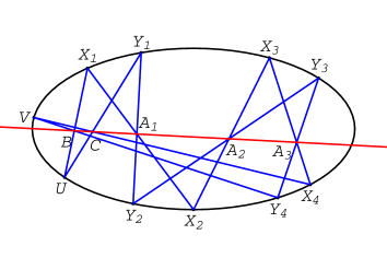
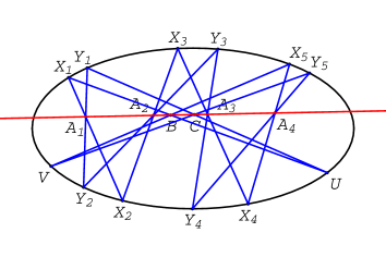
Figure 2: Theorem 2, $N=4,5$

3 Cross-ratio lattice

Here we consider the system of algebraic equations which is equivalent to the collinearity of the intersection points. In this language, Theorems 1, 2 mean that any equation of this system is a consequence of all the others. The derivation of the system is based on the Lemma 3 below. The notation $(a,b,c,d)=(a-b)/(b-c)\cdot(c-d)/(d-a)$ for the cross-ratio is used and, more general, the multi-ratio is denoted as

$$(a,b,\dots,c,d)=(a-b)/(b-\dots)\cdots(c-d)/(d-a).$$

Lemma 3.

1) Let the broken lines $X_{1}X_{2}X_{3}X_{4}$ and $Y_{1}Y_{2}Y_{3}Y_{4}$ be inscribed into a conic section ${\cal C}$, and $x_{j},y_{j}$ be the corresponding values of a rational parameter on ${\cal C}$. Then the collinearity of the intersection points $A_{j}=X_{j}X_{j+1}\cap Y_{j}Y_{j+1}$, $j=1,2,3$ is equivalent to equation

$$(x_{1},y_{2},x_{3},y_{4})=(y_{1},x_{2},y_{3},x_{4}).$$ (1)

2) Let the broken lines $Y_{2}Y_{1}UX_{1}X_{2}$ and $PVQ$ be inscribed into a conic section ${\cal C}$, and $x_{j},y_{j}$, $u,v,p,q$ be the corresponding values of a rational parameter on ${\cal C}$. Then the collinearity of the intersection points

$$A=X_{1}X_{2}\cap Y_{1}Y_{2},\quad B=UX_{1}\cap PV,\quad C=UY_{1}\cap QV$$

is equivalent to equation

$$(p,u,q,x_{2},y_{1},v,x_{1},y_{2})=1.$$

Proof.

Since all nondegenerate conic sections are equivalent modulo projective transformations of the plane, and all birational parametrizations of the conic section are Möbius-equivalent, it is sufficient to check the formulae for some parametrization of some conic section, for example for the parabola $X=(x:x^{2}:1)$. This is a straightforward computation. ∎

It is easy to see that Möbius theorem corresponds to the system

$$(x_{j},y_{j+1},x_{j+2},y_{j+3})=(y_{j},x_{j+1},y_{j+2},x_{j+3}),\quad j=1,\dots,N-2$$ (2)

with the periodic boundary conditions

$$x_{N+1}=x_{1},\quad y_{N+1}=y_{1},\quad N=2n,$$

$$x_{N+1}=y_{1},\quad y_{N+1}=x_{1},\quad N=2n+1.$$

In particular, for $N=3$ the system turns into equation $(x_{1},y_{2},x_{3},x_{1})=(y_{1},x_{2},y_{3},y_{1})$ which is the identity $\infty=\infty$ (Pascal theorem).

For $N=4$ the system consists from equations (1) and $(x_{2},y_{3},x_{4},y_{1})=(y_{2},x_{3},y_{4},x_{1})$ which are obviously equivalent.

In general case, we obtain one more proof of the Möbius theorem by checking that the last equation of the system follows from the others. To this end, notice that the arguments of cross-ratios can be interchanged in arbitrary order, simultaneously in left and right hand sides, and $(a,b,c,d)/(a,b,c,e)=(a,e,c,d)$.

This allows to eliminate $x_{2},y_{2}$ from the first and second equations of the system (2), resulting in $(x_{1},x_{3},y_{4},x_{5})=(y_{1},y_{3},x_{4},y_{5})$. Geometrically, this means that the point $A^{\prime}=X_{1}Y_{3}\cap Y_{1}X_{3}$ is collinear to $A_{3},A_{4}$, so that we follow the proof by recursive applying of Pascal theorem as described in the previous section. On the next step, eliminating $x_{3},y_{3}$ from this new equation and third equation of the system results in equation $(x_{1},y_{4},x_{5},y_{6})=(y_{1},x_{4},y_{5},x_{6})$ which is equivalent to the collinearity of $A^{\prime\prime},A_{4},A_{5}$. Repeat this procedure until come to the equation $(x_{1},x_{N-2},y_{N-1},x_{N})=(y_{1},y_{N-2},x_{N-1},y_{N})$ if $N$ is odd or $(x_{1},y_{N-2},x_{N-1},y_{N})=(y_{1},x_{N-2},y_{N-1},x_{N})$ if $N$ is even, as required.

Analogously, Theorem 2 corresponds to the system

$$(x_{j},y_{j+1},x_{j+2},y_{j+3})=(y_{j},x_{j+1},y_{j+2},x_{j+3}),\quad j=1,\dots,N-3,$$ (3)

$$\left\{\begin{array}[]{ll}(y_{N},u,x_{N},x_{2},y_{1},v,x_{1},y_{2})&=1\\ (y_{1},v,x_{1},x_{N-1},y_{N},u,x_{N},y_{N-1})&=1\end{array}\right.\qquad\mbox{\rm if }N=2n,$$ (6)

$$\left\{\begin{array}[]{ll}(x_{N},u,y_{N},x_{2},y_{1},v,x_{1},y_{2})&=1\\ (y_{1},v,x_{1},y_{N-1},x_{N},u,y_{N},x_{N-1})&=1\end{array}\right.\qquad\mbox{\rm if }N=2n+1$$ (9)

where equations (6) or (9) are equivalent to the collinearity of the points $B,C,A_{1}$ and $B,C,A_{N}$. The ratio of equations (6) is equivalent to equation $(x_{1},y_{2},x_{N-1},y_{N})=(y_{1},x_{2},y_{N-1},x_{N})$ while the ratio of equations (9) is equivalent to $(x_{1},y_{2},y_{N-1},x_{N})=(y_{1},x_{2},x_{N-1},y_{N})$. In both cases, this can be proved to be a consequence of (3).

4 Double cross-ratio equation

Consider in more details Möbius theorem at $N=4$. It says that if three pairs of the corresponding sides of inscribed quadrilaterals $X_{1}X_{2}X_{3}X_{4}$ and $Y_{1}Y_{2}Y_{3}Y_{4}$ meet on a straight line, then the same is true for the fourth pair. As we have seen in the previous section, the figure under consideration is governed by equation (1)

$$(x_{1},y_{2},x_{3},y_{4})=(y_{1},x_{2},y_{3},x_{4}).$$

Due to the transformation properties of cross-ratio this equation can be rewritten in several equivalent forms, so that it provides the collinearity also of several other quadruples of the intersection points (see fig. 3 where one of these additional lines is shown).

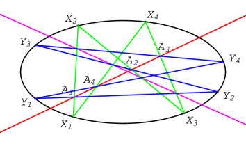
Figure 3: Intersections in a pair of quadrilaterals

In particular, equation (1) is equivalent to $(x_{1},x_{3},y_{2},y_{4})=(x_{4},x_{2},y_{3},y_{1})$ and in this form it express the collinearity of the intersection points of the corresponding sides of the quadrilaterals $X_{1}X_{2}Y_{2}Y_{1}$ and $X_{4}X_{3}Y_{3}Y_{4}$. Another equivalent form $(x_{1},x_{3},y_{4},y_{2})=(x_{2},x_{4},y_{3},y_{1})$ corresponds to the quadrilaterals $X_{1}X_{4}Y_{4}Y_{1}$ and $X_{2}X_{3}Y_{3}Y_{2}$.

In order to make the symmetry between these three forms more explicit, we consider the quadrilaterals $X_{1}X_{2}X_{3}X_{4}$ and $Y_{1}Y_{2}Y_{3}Y_{4}$ as the opposite faces of combinatorial cube and rename them as $XX_{1}X_{12}X_{2}$ and $X_{3}X_{13}X_{123}X_{23}$ respectively. In this notation subscripts correspond to the coordinate shifts $T_{i}:X\to X_{i}$ and their order is unessential, so that $X_{ij}$ and $X_{ji}$ denote the same point. This renumeration brings to the double cross-ratio equation [5, 9]

$$(x,x_{12},x_{13},x_{23})=(x_{123},x_{3},x_{2},x_{1}).$$ (10)

This equation is invariant with respect to any interchange of subscripts and therefore it express the collinearity of the intersection points of the corresponding edges for any pair of the opposite faces of the combinatorial cube.

The double cross-ratio equation is known to be integrable in the sense that it can be self-consistently embedded into a multi-dimensional lattice [1]. This means the following. Consider (10) as a partial difference equation in $\mathbb{Z}^{3}$, so that $x=x(n_{1},n_{2},n_{3})$, $x_{1}=x(n_{1}+1,n_{2},n_{3})$ and so on. Obviously, a generic solution $x:\mathbb{Z}^{3}\to\mathbb{C}\mathbb{P}^{1}$ is uniquely defined by the initial data on the coordinate planes $n_{i}=0$. Now, consider the mapping $x:\mathbb{Z}^{M}\to\mathbb{C}\mathbb{P}^{1}$, $M>3$, governed by equation

$$(x,x_{ij},x_{ik},x_{jk})=(x_{ijk},x_{k},x_{j},x_{i})$$ (11)

for any 3-dimensional sublattice. It turns out that such mapping is also computed from the initial data on the coordinate planes without any contradictions. In order to prove this, it is sufficient to check that if the values $x_{123},x_{124},x_{134},x_{234}$ are found from (11) then equations

$$(x_{l},x_{ijl},x_{ikl},x_{jkl})=(x_{ijkl},x_{kl},x_{jl},x_{il}),\quad\{i,j,k,l\}=\{1,2,3,4\}$$

define one and the same value $x_{1234}$ as function on the initial data $x,x_{1},\dots,x_{34}$. This property is called 4-dimensional consistency. The consistency in the whole $\mathbb{Z}^{M}$ follows. In the next Section we will see that 4-dimensional consistency of double cross-ratio equation is inherited from some more general construction.

5 Quadrilateral lattice on the plane

Double cross-ratio equation defines the mapping from 7 into 1 point on the conic section. If $X,X_{1},\dots,X_{23}$ are given then $X_{123}$ is constructed by means of two most elementary geometric operations only, drawing a line through two points and finding intersection of two lines:

$$\begin{gathered}A^{3}_{1}=XX_{1}\cap X_{3}X_{13},\quad A^{3}_{2}=XX_{2}\cap X_{3}X_{23}\\ A^{3}_{12}=X_{2}X_{12}\cap A_{1}A_{2},\quad A^{3}_{21}=X_{1}X_{12}\cap A_{1}A_{2}\\ X_{123}=A^{3}_{12}X_{23}\cap A^{3}_{21}X_{13}.\end{gathered}$$ (12)

This can be considered also as the mapping from 7 into 1 point on the plane. Möbius theorem guarantees that if initial data lie on a conic section then $X_{123}$ lies on it as well. Moreover, in this case $X_{123}$ does not depend on the interchanging of subscripts in (12), due to the symmetry properties of equation (10), so that three mappings corresponding to the different pairs of the opposite faces actually coincide. The natural question arise, if this is true only for reductions to conic sections, or also for the generic initial data? The answer is given by the following theorem (see fig. 4).

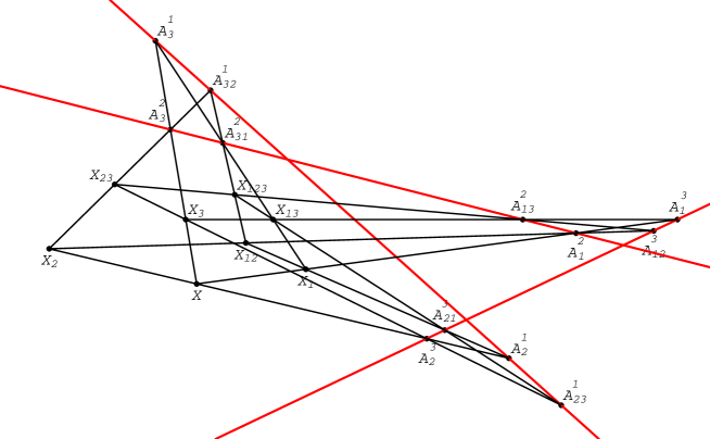
Figure 4: Theorem 4

Theorem 4.

Consider a combinatorial cube on the plane. If, for some pair of the opposite faces, the intersection points of the corresponding edges are collinear, then the same is true for any other pair.

Proof.

As in the case of Desargues theorem, the proof is obtained by constructing a 3-dimensional figure for which the original one is a planar projection. Denote the intersection points as follows:

$$A^{k}_{i}=XX_{i}\cap T_{k}(XX_{i}),\quad A^{k}_{ij}=T_{j}(XX_{i})\cap T_{j}T_{k}(XX_{i}),\quad\{i,j,k\}=\{1,2,3\}$$

and assume that the points $A^{3}_{1},A^{3}_{2},A^{3}_{12},A^{3}_{21}$ are collinear. Let $\alpha$ be the plane of the figure and $\alpha^{\prime}$ be some other plane through the line $A^{3}_{1}A^{3}_{2}$. Choose some point $O$ outside both planes and define the face $X^{\prime}_{3}X^{\prime}_{13}X^{\prime}_{123}X^{\prime}_{23}$ as the projection of the face $X_{3}X_{13}X_{123}X_{23}$ from $O$ onto $\alpha^{\prime}$. All faces of the combinatorial cube $XX_{1}X_{12}X_{2}X^{\prime}_{3}X^{\prime}_{13}X^{\prime}_{123}X^{\prime}_{23}$ are planar. For example, the face $XX_{2}X^{\prime}_{23}X^{\prime}_{3}$ is planar since the lines $X_{3}X_{23}$ and $X^{\prime}_{3}X^{\prime}_{23}$ meet in $A^{3}_{2}$ by construction and this is also the point of intersection of the lines $X_{3}X_{23}$ and $XX_{2}$.

Now, consider the points

$$A^{1}_{2}=XX_{2}\cap X_{1}X_{12},\quad A^{\prime 1}_{3}=XX^{\prime}_{3}\cap X_{1}X^{\prime}_{13},$$

$$A^{\prime 1}_{23}=X^{\prime}_{3}X^{\prime}_{23}\cap X^{\prime}_{13}X^{\prime}_{123},\quad A^{\prime 1}_{32}=X_{2}X^{\prime}_{23}\cap X_{12}X^{\prime}_{123}.$$

They belong to the intersection of the planes $XX_{2}X^{\prime}_{23}X^{\prime}_{3}$ and $X_{1}X_{12}X^{\prime}_{123}X^{\prime}_{13}$ and therefore are collinear. Hence, the points $A^{1}_{2},A^{1}_{3},A^{1}_{23},A^{1}_{32}$ which are the projections of these points from $O$ onto $\alpha$ are also collinear. The collinearity of the points $A^{2}_{1},A^{2}_{3},A^{2}_{13},A^{2}_{31}$ is proved analogously. ∎

Notice that 8 vertices and 12 sides of the cube, 12 intersection points and 3 lines of intersections form a configuration with the symbol $(20_{3}15_{4})$. This configuration is regular, that is, all points and lines are on equal footing. For example, the lines $A^{1}_{2}A^{1}_{23}$ and $A^{2}_{1}A^{2}_{13}$ correspond to the edges of the combinatorial cube with the opposite faces $X_{2}A^{1}_{2}X_{1}A^{2}_{1}$ and $X_{23}A^{1}_{23}X_{13}A^{2}_{13}$, while the lines $XX_{3}$ and $X_{12}X_{123}$ play the role of the lines of intersections for this cube.

The proof of the Theorem 4 makes obvious the link between the mapping (12) and the notion of quadrilateral lattices introduced in [3]. Recall that the $M$-dimensional quadrilateral lattice is a mapping $X:\mathbb{Z}^{M}\to\mathbb{R}^{d}$, $d>2$, such that the image of any unit square in $\mathbb{Z}^{M}$ is a planar quadrilateral $XX_{i}X_{ij}X_{j}$. The image of any unit cube is a combinatorial cube with planar faces. It is clear that the vertex $X_{123}$ in such a figure is uniquely defined as the intersection of the planes

$$X_{123}=X_{1}X_{12}X_{13}\cap X_{2}X_{12}X_{23}\cap X_{3}X_{13}X_{23}$$ (13)

and therefore the 3-dimensional quadrilateral lattice is reconstructed from three 2-dimensional ones corresponding to the coordinate planes which play the role of initial data. The main property of this mapping proved in [3] is its 4-dimensional consistency which guarantees that $M$-dimensional lattice is also reconstructed from 2-dimensional ones without contradiction.

Accordingly to the Theorem 4, the projection of quadrilateral lattice from $\mathbb{R}^{d}$ onto a plane is reconstructed from the images of initial data by applying the mapping (12) instead of (13). Since the quadrilateral lattice in $\mathbb{R}^{d}$ is 4-dimensionally consistent, hence the mapping (12) is 4-dimensionally consistent as well. In particular, this is also true for the reduction of the mapping (12) to a conic section, that is, for double cross-ratio equation (10).

From all above, the following definition of the quadrilateral lattices on the plane can be issued.

Definition.

$M$-dimensional quadrilateral lattice on the plane is a mapping $X:\mathbb{Z}^{M}\to\mathbb{R}^{2}$, $M\geq 3$, such that the images of the corresponding edges of any pair of the opposite faces of any unit cube in $\mathbb{Z}^{M}$ meet on a straight line.

6 Hietarinta equation

Consider the partial difference equation in $\mathbb{Z}^{2}$ introduced by Hietarinta in the recent paper [4] (up to the change $x\to-x$):

$$(x-e^{2})(x_{1}-o^{1})(x_{2}-e^{1})(x_{12}-o^{2})=(x-e^{1})(x_{1}-e^{2})(x_{2}-o^{2})(x_{12}-o^{1})$$

or, as multi-ratio,

$$(x,e^{2},x_{1},o^{1},x_{12},o^{2},x_{2},e^{1})=1.$$ (14)

Here $e^{i},o^{i}$ are parameters of the equation.

Lemma 3 provides the geometric interpretation of this equation as the particular case of Theorem 2 at $N=4$. Like for the double cross-ratio equation, it is convenient to reformulate this case as a mapping from 7 into 1 point on a conic section ${\cal C}$. This mapping is illustrated by the fig. 5 and is described as follows.

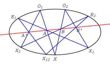
Figure 5: The mapping (15)

Let $X,X_{1},X_{2}$ and $O^{1},O^{2},E^{1},E^{2}$ be points on ${\cal C}$. Then the point $X_{12}\in{\cal C}$ is defined by formulae

$$\begin{gathered}A=XO^{1}\cap X_{1}E^{1},\quad B=XO^{2}\cap X_{2}E^{2}\\ A^{\prime}=X_{2}O^{1}\cap AB,\quad B^{\prime}=X_{1}O^{2}\cap AB\\ X_{12}=E^{1}A^{\prime}\cap E^{2}B^{\prime}.\end{gathered}$$ (15)

The corresponding values of the rational parameter on ${\cal C}$ are related by equation (14).

Equation (14) is 3-dimensionally consistent, that is, the mapping $x:\mathbb{Z}^{M}\to\mathbb{C}\mathbb{P}^{1}$ governed by equation

$$(x,e^{j},x_{i},o^{i},x_{ij},o^{j},x_{j},e^{i})=1$$

for any 2-dimensional sublattice is computed from the initial data on the coordinate axes without contradictions. This can be easily checked directly. At the moment it is not clear, if this property is inherited from some more general construction, as in the case of double cross-ratio equation, and any geometric proof is not known.

Acknowledgment.

I thank A.I. Bobenko and Yu.B. Suris for fruitful discussions and many useful suggestions.

References

- [1] V.E. Adler, A.I. Bobenko, and Yu.B. Suris. Classification of integrable equations on quad-graphs. The consistency approach. Comm. Math. Phys. 233:513–543, 2003.
- [2] A.I. Bobenko, D. Matthes, and Yu.B. Suris, Discrete integrability in geometry and numerics: consistency and approximation. (in preparation)
- [3] A. Doliwa and P.M. Santini. Multidimensional quadrilateral lattices are integrable. Phys. Lett. A 233:265–372, 1997.
- [4] J. Hietarinta. A new two-dimensional lattice model that is “consistent around a cube”. J. Phys. A 37(6):L67–73, 2004.
- [5] B.G. Konopelchenko and W.K. Schief. Three-dimensional integrable lattices in Euclidean spaces: conjugacy and orthogonality. Proc. R. Soc. Lond. A 454(1980):3075–3104, 1998.
- [6] B.G. Konopelchenko and W.K. Schief. Reciprocal figures, graphical statics and inversive geometry of the Schwarzian BKP hierarchy. Stud. Appl. Math. 109(2):89–124, 2002.
- [7] F.A. Möbius. Verallgemeinerung des Pascal’schen Theorems das in einen Kegelschnit beschriebene Sechseck betreffend. J. Reine Angew. Math. 36:216–220, 1848.
- [8] F.W.Nijhoff, A.J.Walker. The discrete and continuous Painlevé hierarchy and the Garnier system. Glasgow Math. J., 2001, 43A, 109–123.
- [9] J.J.C. Nimmo and W.K. Schief. An integrable discretization of a 2+1-dimensional sine-Gordon equation. Stud. Appl. Math. 100(3):295–309, 1998.