Deterministic Bak-Sneppen model. Lyapunov spectrum and avalanches as return times

Abstract

A deterministic version of the Bak-Sneppen model is studied. The role of the Lyapunov spectrum in the onset of scale-free behavior is established and avalanches are interpreted as return times to a zero-measure set. The problem of accurate determination of the scaling exponents near the critical barrier is addressed using a characteristic function approach. A general equation for return times to a small measure set is established and used to obtain information on the nature of Bak-Sneppen dynamics.

1 Introduction

In Ref.[1] several structure-generating mechanisms, in multi-agent dynamical systems, have been analyzed. A structure in a dynamical system is characterized by the emergence of phenomena at scales different from those typical of the dynamics of the agents, when they evolve in isolation. A space-structure corresponds to phenomena operating at a scale much larger than the typical size of one agent and a time-structure is a phenomenon with a time scale much longer than the cycle time of the agents.

An important role in the generation of time-structures is played by modifications to the Lyapunov spectrum, occurring either as a result of the agents’ interaction or of a change of parameters. A new structure is created each time one Lyapunov exponent crosses zero from above. In particular, in one of the mechanisms described in [1], the joint effect of chaos in the individual agent evolution law and extremal dynamics, implies that all Lyapunov exponents tend to $0^{+}$ in the infinite agents limit. This leads to a characteristic behavior free of time scales. It has been conjectured in Ref.[1] that it is this mechanism that is behind many of the dynamical manifestations of what has been called self-organized criticality (SOC). Here, this conjecture is pursued by analyzing a situation [2] where breakdown of self-organized criticality is exhibited. It is shown that the breakdown of SOC may in fact be understood from the behavior of the Lyapunov spectrum.

There is some controversy concerning a rigorous definition of SOC. Here only the absence of natural time scales is emphasized, without much concern about space scales, nature of the driving, separation of time scales and other relevant issues useful for a precise characterization of SOC.

Absence of time scales, as a property of dynamics, is naturally related to the Lyapunov spectrum. Time scales disappear whenever the Lyapunov exponents vanish. This leads in a natural way to power laws for both time and space correlation. However, scaling of the avalanches, that is, a power law for the return times to the self-organized state, is a subtler effect. This is easy to understand when the multi-agent system is formulated as a measure-preserving dynamical system. If the self-organized state $A$, which serves as reference for the counting of return times $\left(k\right)$, is a non-zero measure set $\left(\mu\left(A\right)\neq 0\right)$, the measure $\mu\left(A\right)$ itself serves as a natural time scale. Then, the large time behavior of the return times distribution would be dominated by an exponential factor $\exp\left(-k\nu\left(\mu\right)\right)$. Therefore, for cases that fit in the ergodic dynamical systems setting, power laws may occur only if the reference set has vanishing measure. In the $\mu\left(A\right)\rightarrow 0$ limit the return times distribution is dominated by the pre-factor that multiplies the exponential and this one might be or not be a power law.

When $\mu$ is an ergodic measure, by Kac’s lemma, the mean return time to a set $A$ is $1/\mu\left(A\right)$. Therefore when $\mu\left(A\right)=0$, the numerical evaluation of the return time (avalanche) law has to be carried out for a set slightly larger than $A$. This implies that it may be difficult to disentangle the prefactor dependence from the exponential one, leading to some uncertainty about the exact values of the numerically measured scaling exponents. In particular because, as seen in Sect. 2, the exponent factor $\nu\left(\mu\right)$ may be a non-trivial function of the measure. Instead of obtaining the return times distribution from the histogram, a more robust way is described in Sect.2, based on the construction of the characteristic function.

Treating the multi-agent system as a deterministic measure-preserving dynamical system, tools from ergodic theory may be applied. An important issue is the characterization of asymptotic sets and invariant measures as well as the nature of the relevant attractors and repellers of the scale-free system. These questions are discussed for a deterministic version of the Bak-Sneppen model[3]. The nature of the self-organized state as a zero-measure subset of the invariant measure is put into evidence. Then, a probabilistic avalanche equation, written for the return times, is used to extract the non-trivial nature of the avalanche process from simulation data.

2 The deterministic Bak-Sneppen model

The original Bak-Sneppen model [3] [4] may be converted into a deterministic dynamical system by defining

$$x_{i}\left(t+1\right)=\Gamma_{i}\left(\underset{\sim}{x}\right)x_{i}\left(t\right)+\left(1-\Gamma_{i}\left(\underset{\sim}{x}\right)\right)f\left(x_{i}\left(t\right)\right)$$ (1)

where $\underset{\sim}{x}=\left\{x_{i}\right\}$ is the vector of agent coordinates and $f$ a deterministic pseudo-random generator, for example

$$f\left(x_{i}\right)=kx\hskip 28.45274pt\textnormal{mod}.1$$

$k=2,3,\cdots$ . $\Gamma_{i}\left(\underset{\sim}{x}\right)$ is a function which is nearly zero if $i$ corresponds to the agent with the minimum $x_{i}$ value or to one of its $2n_{v}$ neighbors and is nearly one otherwise. In Ref.[1] the following function was proposed

$$\Gamma_{i}^{(1)}\left(\underset{\sim}{x}\right)=\prod_{j=i-n_{V}}^{j=i+n_{V}}\left(1-\prod_{l\neq j}\left(1+e^{-\alpha\left(x_{l}-x_{j}\right)}\right)^{-1}\right)$$ (2)

which, for large $\alpha$, satisfies the above conditions.

Here, instead, the function

$$\Gamma_{i}^{(2)}\left(\underset{\sim}{x}\right)=\prod_{j=i-n_{V}}^{j=i+n_{V}}\left(1-\frac{e^{-x_{j}/T}}{\sum_{l=1}^{N}e^{-x_{l}/T}}\right)$$ (3)

will be used, which has a similar behavior for $T\rightarrow 0^{+}$. Using a similar function in a stochastic model Head[2] has shown the breakdown of scale-free behavior for finite non-zero $T$. By using $\Gamma_{i}^{(2)}\left(\underset{\sim}{x}\right)$ in the deterministic model one may compare the Lyapunov spectrum analysis with the numerical results of Head. In the $T\rightarrow 0$ limit both models are equivalent to the original Bak-Sneppen model.

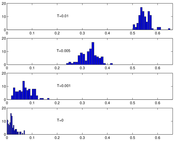
Figure 1: Approximate Lyapunov spectrum for several $T$ values in the deterministic Bak-Sneppen model

Fig.1 shows an approximate calculation of the evolution of the Lyapunov spectrum for successively decreasing $T$ values with $N$ agents. The results were obtained for $N=100$, $1000$ time steps and $2n_{V}=2$. The spread in the $T=0$ limit, around the exact value for $N$ agents $\left(\frac{3}{N}\log 2=0.02\text{ in this case}\right)$, results from the finite number of time steps. The deterministic system defined by (1)-(3) closely corresponds to the stochastic system studied in Ref.[2]. Therefore the behavior of the Lyapunov spectrum explains why the distribution of jump sizes and activation times obeys power laws only in the $T\rightarrow 0$ limit. In Ref. [2] the loss of criticality for finite $T$ is interpreted in terms of the correlated or uncorrelated nature of the active site jumps. The Lyapunov spectrum interpretation is clearer. Notice also that it is only in the $N\rightarrow\infty$ limit that all the Lyapunov exponents reach $0^{+}$. It is only in this limit that all time scales disappear [1].

One of the most remarkable features of the Bak-Sneppen model is the existence of a sharp probability distribution for the agents coordinates above a barrier $b\simeq 0.667$. However, this sharp (full-measure) distribution is merely a fixed point for the one-agent marginal, which is the one-dimensional projection of a zero-measure subset of the invariant measure in the $N-$ dimensional space [1]. The fact that in the $N-$dimensional space the self-organized set to which the system returns after each avalanche is of zero measure is consistent with Kac’s lemma. Kac’s lemma states that for an ergodic invariant measure $\mu$ the average return time to a set $A$ of measure $\mu\left(A\right)$ is $1/\mu\left(A\right)$. Therefore for a scaling law $\rho\left(k\right)\sim 1/k^{\tau}$, $\tau\leq 2$ implies $\mu\left(A\right)=0$.

To exhibit the zero-measure nature of the Bak-Sneppen state consider the distance process $d$ defined by

$$d=\sum_{i}\max\left(b-x_{i},0\right)$$ (4)

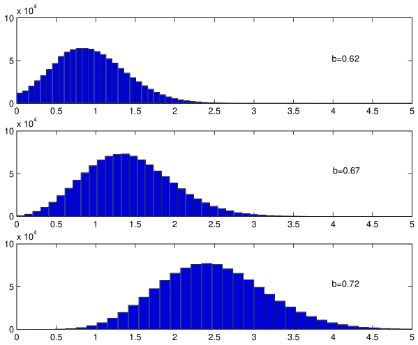
Figure 2: Probability density for the distance process

Fig.2 shows the probability distribution of the distance process for several values of the barrier $b$. One sees that it is for $b$ around $0.67$ that the neighborhood of the $d=0$ point becomes of zero measure.

The Bak-Sneppen self-organized state is an $N-$dimensional hypercube of volume $\left(1-0.667\right)^{N}$. This set has repelling directions corresponding to the agents that are active and neutral directions for all others. Not being an invariant set it falls outside the usual definition of “weak repeller”. It has been called a “ghost weak repeller” in Ref. [1].

As mentioned before, the zero measure of this “repeller” makes the direct measurement of the distribution law of avalanches a delicate matter. On the one hand the barrier value defining the avalanches must be placed close to the critical barrier to avoid the exponential finite-measure effects. However because the average size of the avalanches is $1/\mu\left(A\right)$, the closer we are to the critical barrier the worse the statistics becomes. A bin size has to be chosen to fit the avalanches data to a power law and the accuracy of the exponent is found to be sensitive to the bin size.

Logarithmic binning may improve the situation. However a more robust method is based on the construction of the characteristic function

$$C\left(x\right)=\left\langle e^{ikx}\right\rangle$$ (5)

from the data. For each avalanche size $k$, the probability density may then be obtained by numerical computation of the inverse Fourier transform

$$p\left(k\right)=\frac{1}{2\pi}\int_{-\pi}^{\pi}C\left(x\right)e^{-ikx}dx$$ (6)

In this way all the data is used for each $k$ instead of only the events in the neighborhood of $k$.

For sparse data this is a very robust way to construct $p\left(k\right)$, which is no longer affected by the bin size choice. However in our case we are not only interested in an accurate determination of $p\left(k\right)$ but also on the extraction of the power law prefactor that multiplies the measure-dependent exponential. In cases where the exponent of the exponential is also a non-trivial function of the measure it is extremely difficult to separate the effect of the two terms. This is especially true if the measure-dependent exponent decreases with the measure (see the example below).

More accurate statements, concerning the nature of the prefactors, are obtained by comparing the characteristic function constructed from the data with the characteristic functions for trial distributions

$$p\left(k,\mu\right)=ck^{-\alpha\left(\mu\right)}e^{-\nu_{\alpha}\left(\mu\right)k}$$ (7)

with $c$ and $\nu_{\alpha}\left(\mu\right)$obtained from normalization and Kac’s lemma, $\left\langle k\right\rangle=\frac{1}{\mu}$ . This was done for several values of the measure, the results being displayed in Fig.3 (for $2n_{v}=2$). Both the exponential factor $\nu$ and the scaling exponent $\alpha$ depend on the measure of the avalanche reference set.

Figure 3: The exponential argument $\nu(\mu)$ and scaling exponent $\alpha(\mu)$

This puts into evidence the unavoidable uncertainties in the direct evaluation of the scaling exponent, in particular because even very close to the critical barrier the scaling exponent still shows a noticeable dependence on the measure of the reference set. In the Appendix the characteristic functions associated to the probability distributions in Eq.(7) are discussed in detail as well as some other results concerning return times to small measure sets.

The discussion above refers to the problem of direct determination of the scaling exponents. However, with the additional assumption, as done by several authors, of a scaling form for $p\left(k\right)$ near the critical barrier, an estimate of the $\mu\rightarrow 0$ value may be obtained. This however relies on the validity of the scaling assumption. Assuming that close to $\mu=0$

$$p\left(k,\mu\right)=k^{-\alpha}f\left(k^{s}\mu\right)$$ (8)

one obtains

$$\begin{array}[]{lll}\left\langle k\right\rangle&\sim&\mu^{\frac{\alpha-2}{s}}\\ \left\langle k^{2}\right\rangle&\sim&\mu^{\frac{\alpha-3}{s}}\end{array}$$ (9)

Then, from Kac’s lemma, one obtains

$$s=2-\alpha$$

and from the numerical data for $2n_{v}=2$ (Fig. 4a), $\frac{\alpha-3}{s}\simeq 2.07$, leading to $\alpha\simeq 1.067$, $s\simeq 0.93$.

Figure 4: Data points used to infer the exponents in $\left\langle k^{2}\right\rangle\sim\mu^{\frac{\alpha-3}{s}}$ and $\mu\sim\left(b_{c}-b\right)^{\eta}$

Another exponent relates the measure to the position of the barrier

$$\mu\sim\left(b_{c}-b\right)^{\eta}$$

with (Fig. 4b) $\eta\simeq 2.55$.

3 The avalanche equation

Assuming a differentiable dependence of the avalanches on the position of the barrier, Maslov [5] derived an equation for the probability density of avalanche sizes in the Bak-Sneppen model. Here, a similar equation will be obtained for the return times to a measure $\mu$ set. This equation is then applied to the Bak-Sneppen model. Particular attention is paid to the avalanche merging kernel, which in the Maslov equation is usually assumed to scale like a power in the critical region, but that may actually have a much more complex form.

Assume that a set parametrization may be chosen in such a way that set measures change in a differentiable manner. Differentiating with respect to the measure, one obtains the following equation

$$dp\left(k\right)=p\left(k\right)\left(2\gamma\left(k,\mu\right)d\mu-\frac{d\mu}{\mu}\right)-\sum_{j=1}^{k-1}p\left(j\right)\gamma\left(j,\mu\right)d\mu p\left(k-j\mid j\right)$$ (10)

where

$$P\left(T^{A\rightarrow A}=k,\mu\left(A\right)\right)\doteq p\left(k\right)$$

Eq.(10) is derived by shrinking the measure of the set $A$ by the amount $d\mu$ and accounting for the number of avalanches of size $k$ that become avalanches of larger size and for the number of mergers of smaller avalanches leading to new $k-$avalanches. $\gamma\left(k,\mu\right)d\mu$ is the probability that the first or the last step of a $k-$avalanche iteration falls in $d\mu$. The first term in Eq.(10) accounts both for a $k-$avalanche becoming a larger avalanche and for the change in the total number of events from $N$ to $N\left(1+\frac{d\mu}{\mu}\right)$. The second term accounts for the probability for a $j-$avalanche and a $\left(k-j\right)-$avalanche to merge into a $k-$avalanche. $p\left(k-j\mid j\right)$ is the conditional probability to have a $\left(k-j\right)$ avalanche following a $j$ one.

With the additional hypothesis of statistical independence between successive avalanches

$$p\left(k-j\mid j\right)=p\left(k-j\right)$$ (11)

Defining $C\left(x,\mu\right)=\left\langle\exp\left(ikx\right)\right\rangle$ (the characteristic function) and $Q\left(x,\mu\right)=\left\langle\gamma\left(k,\mu\right)\exp\left(ikx\right)\right\rangle$ one obtains

$$\frac{d}{d\mu}C\left(x,\mu\right)=2Q\left(x,\mu\right)-\frac{1}{\mu}C\left(x,\mu\right)-Q\left(x,\mu\right)C\left(x,\mu\right)$$ (12)

So far this is a very general equation that (with statistical independence of avalanches) would apply to any dynamical system. The dynamical information of each system is coded on the “merging kernel” $\gamma(k,\mu)$. Using normalization $\left(C\left(0,\mu\right)=1\right)$ and Kac’s lemma $\left(-i\frac{d}{dx}C\left(x,\mu\right)\mid_{x=0}=\frac{1}{\mu}\right)$ in Eq.(12) one obtains the following constraints on $\gamma(k,\mu)$

$$\begin{array}[]{lll}\left\langle\gamma(k,\mu)\right\rangle&=&\frac{1}{\mu}\\ \left\langle k\gamma(k,\mu)\right\rangle&=&\frac{1}{\mu^{2}}\end{array}$$ (13)

A trivial solution to the constraints (13) is

$$\gamma(k,\mu)=\frac{1}{\mu}$$ (14)

leading to the equation

$$\mu\frac{dC\left(x,\mu\right)}{d\mu}=C\left(x,\mu\right)-C^{2}\left(x,\mu\right)$$ (15)

with solution

$$C\left(x,\mu\right)=\frac{\mu}{\mu+q\left(x\right)}$$ (16)

with $q\left(0\right)=0$ and $q^{{}^{\prime}}\left(0\right)=-i$, from normalization and Kac’s lemma. Otherwise $q\left(x\right)$ is an arbitrary function of $x$.

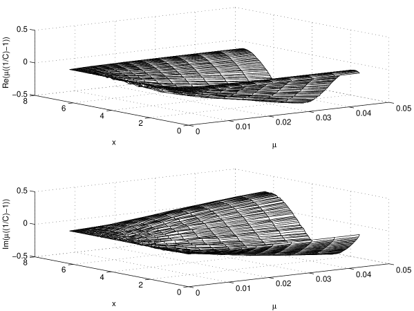
Figure 5: Real and imaginary parts of $\mu\left(\frac{1}{C(x,\mu)}-1\right)$

However the Bak-Sneppen model is not in the class of solutions (16), because from this equation it follows that $\mu\left(\frac{1}{C\left(x,\mu\right)}-1\right)$ should be independent of $\mu$, which is not verified by the numerical data (Fig. 5).

A power dependence of the merger kernel $\gamma(k,\mu)$

$$\gamma(k,\mu)=\alpha_{1}\frac{1}{\mu}+\alpha_{2}k^{\varepsilon}$$

together with the constraints (13) implies

$$\left\langle k^{\varepsilon}\right\rangle_{\mu}=\mu\left\langle k^{\varepsilon+1}\right\rangle_{\mu}$$

which again, is not borne out by the data.

However from the numerical simulation data ($2n_{v}=2$) for two close values of the measure and Eq.(12) one may obtain direct information on $\gamma(k,\mu)$ from

$$\gamma(k,\mu)=\frac{\int_{-\pi}^{\pi}Q\left(x,\mu\right)\exp\left(-ikx\right)dx}{\int_{-\pi}^{\pi}C\left(x,\mu\right)\exp\left(-ikx\right)dx}$$

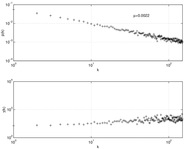
Figure 6: $p(k)$ and $\gamma(k)$ for $\mu=0.0022$

An example is shown in Fig. 6, where both $p\left(k,\mu\right)$ and $\gamma\left(k,\mu\right)$ are plotted. The general conclusion from these computations for several measures is that, starting from a non-zero value at $k=1$, $\gamma\left(k,\mu\right)$ grows relatively fast to the asymptotic value $\frac{1}{\mu}$. A (weak) power dependence is only found for small $k$ values. Therefore the behavior of the merger kernel, that codes the dynamical information of the Bak-Sneppen model, seems to be much more complex than thought before.

4 Conclusions

(i) The deterministic Bak-Sneppen model, studied in this paper, establishes a clear relation between the Lyapunov spectrum and scale-free behavior.

Extremal behavior, where only a finite number of agents is active at each time, leads to the vanishing of all Lyapunov exponents in the infinite agents limit. On the other hand, local chaos insures that the convergence to zero is from above. These seem to be the most common ingredients in systems that display what has been called self-organized criticality.

(ii) The self-organized state in the deterministic Bak-Sneppen model is an interesting zero-measure subset of the invariant measure. Interpreting avalanches as return times to a set $A$, one concludes that a scaling law with exponent $\leq 2$ implies, by Kac’s lemma, $\mu\left(A\right)=0$. Therefore one expects the zero measure feature to be present not only in the Bak-Sneppen model but also in other self-organized states with avalanche scaling laws.

(iii) The avalanche equation, in the measure formulation discussed in Section 3, is a powerful guide to constraint the extraction of dynamical information from dynamical systems of this type. In particular it provides preliminary evidence on a non-power behavior of the merger kernel. A stretched exponential behavior converging to $\frac{1}{\mu}$ seems to be a better guess. This however is a question that deserves further study.

5 Appendix. Return times to small measure sets

On a measurable space $\left(M,{\cal B},\mu\right)$, consider a differentiable map $T$ for which $\mu$ is an ergodic invariant measure. The return time $\tau_{A}\left(x\right)$ to a measurable set $A$ starting from a point $x\in M$ is

$$\tau_{A}\left(x\right)=\inf\left\{\left(k\geq 1\mid T^{k}x\in A\right)\cup\infty\right\}$$ (17)

The probability to find a return time greater than $k$, starting from an arbitrary point $x\in M$

$$P\left(T^{M\rightarrow A}>k\right)=\mu\left(\tau_{A}\left(x\right)>k\right)$$ (18)

and for a starting point $x$ in $A$

$$P\left(T^{A\rightarrow A}>k\right)=\mu_{A}\left(\tau_{A}\left(x\right)>k\right)$$ (19)

where

$$\mu_{A}\left(\tau_{A}\left(x\right)>k\right)=\frac{\mu\left(A\cap\left\{\tau_{A}\left(x\right)>k\right\}\right)}{\mu\left(A\right)}$$ (20)

Invariance of the measure implies

$$\mu\left(\tau_{A}\left(x\right)>k\right) = \mu\left(A^{c}\cap\left\{\tau_{A}\left(x\right)>k-1\right\}\right)$$

$$= \mu\left(\tau_{A}\left(x\right)>k-1\right)-\mu\left(A\right)\mu_{A}\left(\tau_{A}\left(x\right)>k-1\right)$$

and because $P\left(T^{M\rightarrow A}=k\right)=\mu\left(\tau_{A}\left(x\right)>k-1\right)-\mu\left(\tau_{A}\left(x\right)>k\right)$

$$P\left(T^{M\rightarrow A}=k\right)=\mu\left(A\right)P\left(T^{A\rightarrow A}>k-1\right)$$ (22)

Because of ergodicity, Poincaré recurrence implies $\sum_{k=1}^{\infty}P\left(T^{M\rightarrow A}=k\right)=1$. On the other hand $\sum_{k=1}^{\infty}P\left(T^{A\rightarrow A}>k-1\right)=\sum_{k=1}^{\infty}kP\left(T^{A\rightarrow A}=k\right)$ and for $\mu\left(A\right)\neq 0$ one obtains Kac’s lemma

$${\mathbb{E}}\left(\tau_{A}\left(x\right)\mid x\in A\right)=\int_{A}\tau_{A}\left(x\right)d\mu_{A}\left(x\right)=\frac{1}{\mu\left(A\right)}$$ (23)

Defining, as in [6]

$$c\left(k,A\right)=\mu_{A}\left(\tau_{A}\left(x\right)>k\right)-\mu\left(\tau_{A}\left(x\right)>k\right)$$ (24)

one obtains from (5) and (19)

$$P\left(T^{A\rightarrow A}>k\right)=\left(1-\mu\left(A\right)\right)P\left(T^{A\rightarrow A}>k-1\right)-\Delta c\left(k,A\right)$$

where $\Delta c\left(k,A\right)=c\left(k-1,A\right)-c\left(k,A\right)$. By iteration

$$P\left(T^{A\rightarrow A}>k\right)=\left(1-\mu\left(A\right)\right)^{k}-\sum_{j=1}^{k}\Delta c\left(j,A\right)\left(1-\mu\left(A\right)\right)^{k-j}$$ (25)

Let

$$\Delta c\left(A\right)=\sup_{k}\left|\Delta c\left(k,A\right)\right|$$ (26)

Then, by standard techniques, as in [6], one obtains the estimation

$$\left|P\left(T^{A\rightarrow A}>k\right)-e^{-k\mu\left(A\right)}\right|\leq 2\mu\left(A\right)+\Delta c\left(A\right)\left(1-\log\Delta c\left(A\right)\right)$$ (27)

This estimate is sharper than the one obtained in [6] because it involves $\Delta c\left(A\right)$ rather than $c\left(A\right)=\sup_{k}\left|c\left(k,A\right)\right|$.

The estimate (27) holds whenever $\mu\left(A\right)\neq 0$. However it is useless to find $p(k,\mu)=P\left(T^{A\rightarrow A}=k\right)$ in the $\mu\left(A\right)\rightarrow 0$ limit because

$$e^{-\left(k-1\right)\mu\left(A\right)}-e^{-k\mu\left(A\right)}=e^{-k\mu\left(A\right)}\left(e^{-\mu\left(A\right)}-1\right)\underset{\mu\left(A\right)\rightarrow 0}{\rightarrow}0$$

Therefore, a different approach must be followed to control the $\mu\left(A\right)\rightarrow 0$ limit.

For general distributions of the form

$$p_{g}\left(k,\mu\right)\sim g\left(k\right)e^{-k\nu\left(\mu\right)}$$

the characteristic function must satisfy the equation

$$\frac{d}{d\nu}C\left(x,\mu\right)=i\frac{d}{dx}C\left(x,\mu\right)+\frac{1}{\mu}C\left(x,\mu\right)$$

with solution

$$C\left(x,\mu\right)=\exp\left(\int_{\nu_{0}}^{\nu}\frac{d\tau}{\mu\left(\tau\right)}-\int_{\nu_{0}}^{\nu-ix}\frac{d\tau}{\mu\left(\tau\right)}\right)$$

Therefore a large family of solutions is obtained simply by specifying the function $\nu\left(\mu\right)$ (and its inverse $\mu\left(\nu\right)$).

A particular case is

$$p_{\alpha}\left(k,\mu\right)\sim k^{-\alpha}e^{-k\nu_{\alpha}\left(\mu\right)}$$

For $\alpha=0$ this is the geometric distribution with

$$\nu_{\alpha}\left(\mu\right)=-\log\left(1-\mu\right)$$

and for $\alpha=1$

$$C_{1}\left(x,\mu\right)=\frac{\log\left(1-\exp\left(ix-\nu\right)\right)}{\log\left(1-\exp\left(-\nu\right)\right)}$$

with

$$\mu=\left(1-e^{\nu}\right)\log\left(1-e^{-\nu}\right)$$

The functions $\nu_{\alpha}\left(\mu\right)$ for other values of $\alpha$ are plotted in Fig.7.

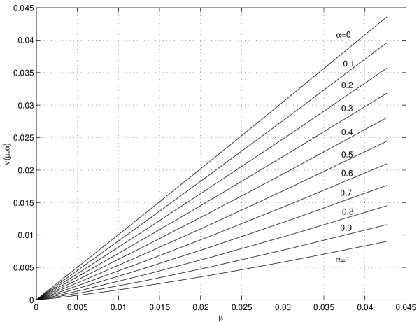
Figure 7: Exponential argument $\nu_{\alpha}(\mu)$ for the probability densities $p_{\alpha}\left(k,\mu\right)\sim k^{-\alpha(\mu)}\exp\left(-k\nu_{\alpha}(\mu)\right)$

References

- [1] R. Vilela Mendes; Physica A295 (2001) 537.
- [2] D. Head; Eur. Phys. Journal B17 (2000) 289.
- [3] P. Bak and K. Sneppen; Phys. Rev. Lett. 71 (1993) 4083.
- [4] H. Flyvbjerg, K. Sneppen and P. Bak; Phys. Rev. Lett. 71 (1993) 4087.
- [5] S. Maslov; Phys. Rev. Lett. 77 (1996) 1182.
- [6] M. Hirata, B. Saussol and S. Vaienti; Commun. Math. Phys. 206 (1999) 33.