Dynamic Domain Networks

Abstract

We present a model for the description of the evolution of contacts among individuals in a network. At each time step each individual is associated with a domain or neighborhood of fully connected agents.The dynamics of this changing neighborhood will later be translated into a situation where the links between individuals are also dynamic. A characterization in terms of the parameters that govern the evolution of the network and a comparison to previous work on Small World networks is presented as well.

I Introduction

The study of networks and their applications within social sciences has in recent years been a rich source of interdisciplinary research. In particular, development of mathematical models based on simple social interactions formulated with graphs or networks, with certain topological properties, has accumulated much interest. The concept of the small world was first introduced by Milgram milgram in an attempt to describe the intrinsic properties of social communities and the relationships that exist amongst the members thereof. A more mathematical approach was later introduced to understand the underlying aspects of Milgram’s networks watts98 . Small World Networks (SWN) are in essence, those networks which are comprised of a specified amount of random and regular lattice connections. Driven by strong evidence that certain complex networks share a close resemblance with actual economic, social, and biological networks, a new field has been developing within physics stro . Such real world applications have naturally led to the proposition of temporally evolving networks ama ; albe . We will refer to dynamic networks as those which rewire links as time progresses. Networks in which the links remain static in time once the desired architecture has been achieved, are known as quenched networks. Whereas networks with links that change randomly at every time step are called annealed networks. An example of the latter, which is akin to the model developed here, may be found in manr . The model we present consists of subnetworks which are only linked to each other through time. A dynamic domain network (DDN) is thus a type of annealed network, though at a given moment the subnetworks or domains are not connected to each other. As explained in the next section, the model we propose may be associated with a phenomena where the only mechanism of transmission or propagation throughout the network is a type of diffusion. Though the model can be generalized to include other features such as long range transmission (as found in SWNs), we are for now interested in analyzing properties due solely to this specialized diffusion. The possibility of analyzing different dynamic degrees of freedom independently will lead to a deeper understanding of diffusion within networks. In the following sections we will consider in more detail the features guiding our analysis,

• Two measurable parameters, $\omega$ and $\tau$, which may be associated with the SWN parameters, clusterization and average path length.

• Three types of domain movement, $p_{d}$, $p_{f}$, and $p_{s}$, which are called the dynamic processes of the system, are analyzed

• Numerical analysis and limited analytic calculation of $\omega$ and $\tau$ as functions of the dynamic processes demonstrate common characteristics with SWNs.

• Diffusion coefficients associated with each dynamic process are numerically and analytically calculated.

• The DDN model reproduces features found in previous work on disease propagation and further shows the affect of each dynamic process on the total population infection.

II The model

The model is based on a two dimensional array of individuals, each one situated on the node of a matrix of size $n\times n$. The system is divided into $N$ domains, or fully connected subnetworks, of size $k^{2}$. In what we call the regular case, all domains have the same shape and size. We consider that an individual is linked to the other individuals belonging to the same domain, but not to the rest of the system. The boundaries that demarcate the domains change in time and thus may be considered as independent neighborhoods exchanging members through dynamic links in time. The architecture of the underlying dynamic network is defined by the history of the changes of the boundaries. A set of three processes govern the behavior of these domains and thus three different parameters will be considered. At each time step the whole set of domains may be displaced or shifted from their former positions with probability $p_{d}$. It is also possible that domains change individual size with probability $p_{s}$ and change form or shape with probability $p_{f}$. Each of these processes can act separately, but when all three take place at the same time, a superposition of their effects occur. To characterize some of the dynamic properties of the evolving network we have chosen a few observable quantities as suggested in manr . We consider a measurable global variable analogous to the average path length in SWNs. Over all domains and throughout time, we analyze the time necessary for an ‘active’ state to propagate across the entire system. Initially, one individual is chosen to be active. Any inactive individual in the same domain is immediately activated by the presence of at least one active individual in the same neighborhood. Once activated, the individual remains as such for all time. We measure the time involved $\tau_{i}$, to activate the node $i$ within the system. The mean persistence or activation time $\tau$, is calculated as defined in manr . This value is studied for different sets of $p_{d}$, $p_{s}$, and $p_{f}$. As a second characterization of the system, we analyze the changes in the composition of each individual’s domain from one time step to another. Again, in accordance with manr , this local measurable variable may be associated with a clustering coefficient watts98 . As a general definition we call $\omega_{i}(t)$ the overlap or intersection of domains during $m$ consecutive time steps, where in the present work $m=2$. The mean neighborhood overlap is then calculated for varying values of $p_{d}$, $p_{s}$, and $p_{f}$. Compared to previous models of dynamic networks, this model may be associated with diffusive processes. This supposition will be reinforced with the calculation of associated diffusion constants.

III Analytic considerations

As a measure of the common area of two domains between consecutive time steps, the overlap may be written analytically in a general form. In the model we have considered that the allowable sizes take on only quadratic values so that the square shape is always accessible, particularly for the case when the form does not change at all. We thus compare all possible forms of the permitted sizes between a before domain and an after domain. The expression for the mean overlap for any set of values $\overline{p}=(p_{d},p_{s},p_{f})$ can be written in general as a binomial distribution

$${\omega(\overline{p})} = \sum_{i=0}^{2}\,\sum_{j=0}^{2}\,\sum_{k=0}^{2}\binom{2}{i}\binom{2}{j}\binom{2}{k}$$

$$a_{ijk}(\overline{p})p_{d}^{i}(1-p_{d})^{2-i}p_{s}^{j}(1-p_{s})^{2-j}p_{f}^{k}(1-p_{f})^{2-k}$$

The coefficients $a_{ijk}(\overline{p})$ must be calculated by considering the superposition for any succession of two allowed states of the system for a given set of values $\overline{p}$. Since we preserve the rectangular shape of the domains, the overlap is determined by the divisors of domain sizes in the before and after configurations. This allows us to write a counting scheme for the overlap when $p_{d}=0$.

$$\frac{\sum_{m=\alpha}^{n}\sum_{k=\alpha}^{n}\left[\sum_{i=\gamma_{m}}^{N_{m}}\sum_{j=\gamma_{k}}^{N_{k}}s_{ij}s_{(N_{m}-i+1)(N_{k}-j+1)}\frac{1}{N_{m}N_{k}}\right]}{(n-\alpha+1)^{2}}.$$ (2)

With this, the overlap is calculated for the four extreme situations when $p_{s}$ and $p_{f}$ are either zero or one. The parameters $N_{m}$ and $N_{k}$ indicate the number of divisors of the sizes $m^{2}$ and $k^{2}$, for each before and after domain, respectively. The value $n^{2}$ is the maximum size allowed. To calculate the case when $p_{s}=p_{f}=1$, one must set $\alpha=\gamma_{m}=\gamma_{k}=1$; this sums over all forms and all sizes bounded by $n$. For zero change in form and size $p_{s}=p_{f}=0$, the parameters must be set to $\alpha=n$, $\gamma_{m}=\frac{N_{m}-1}{2}+1$, and $\gamma_{k}=\frac{N_{k}-1}{2}+1$. Changes in size $p_{s}=1$, and no change in form $p_{f}=0$ correspond to $\alpha=1$, $\gamma_{m}=\frac{N_{m}-1}{2}+1$, and $\gamma_{k}=\frac{N_{k}-1}{2}+1$. Changes in form $p_{f}=1$, and no change in size $p_{s}=0$, correspond to $\alpha=n$ and $\gamma_{m}=\gamma_{k}=1$. These extreme values define four of the eight coefficients in Eq. III.

The underlying diffusive process occurring in the network as time proceeds is another interesting feature we would like to address. We begin by considering one particle located within an initial domain. This test subject then performs a walk to neighboring domains as the domain walls change and an overlap between the original domain and a neighboring one permit movement of the individual. Indeed, the process may be considered as a random walk, characterized by a probability distribution particular to each dynamic process. A brief analysis of what movement might be expected can be done by considering the possibilities of change associated with each process. As an example, consider the case of a dynamic domain originally comprised of nine sites. A probability can be calculated for a given random walker located at the center of the original domain to step to the center of one of the neighboring domains with which it overlaps in a given time step. Two different jumps should be considered; those to neighboring domains that share a side with the original one, and those to any of the other four domains along the diagonals. We will call $\alpha$ the probability of the first type of jump, and $\beta$ the probability corresponding to jumps of the second type. The $\alpha$ and $\beta$ probabilities for each of the three processes can be calculated by considering the fractions of all the overlap situations that will lead to a given jump, where we have calculated $\alpha_{d}=0.12$, $\beta_{d}=0.04$, $\alpha_{s}=0.024$, $\beta_{s}=1/256$, $\alpha_{f}=1/9$, $\beta_{f}=0$. These values are used to evaluate a random walk process and thus an associated diffusion coefficient.

A random walker in one dimension with equal likeliness to jump to the right or left is analyzed. This probability to move is given by $p(\alpha+2\beta)$, where $\alpha$ and $\beta$ correspond to the values mentioned previously and $p$ is the value characterizing the probability for a change in the position, size, or shape. Further, there is a probability to stay in the same site, $\gamma=1-p(2\alpha+4\beta)$. This leads to a calculation of the mean square displacement $\langle x^{2}\rangle$, of a set of particles equal to $18p(\alpha+2\beta)t$ manuel . By considering the appropriate values for each dynamic process, we find that the diffusion coefficients for each are given by $D_{d}=1.8p_{d}$, $D_{s}=0.28p_{s}$ and $D_{f}=p_{f}$.

IV Numerical results

Extensive numerical simulations of the described model for networks of $n^{2}=10^{4}$ to $10^{7}$ nodes and $k=3$ to $10$ have been performed. A typical realization starts with the random election of an active individual. In the successive time steps, the active condition propagates throughout the system until the system is entirely activated. We calculate the mean activation time of the system as

$${\tau}=\frac{1}{n^{2}}\sum_{i=1}^{n^{2}}\tau_{i},$$

where $\tau_{i}$ is the activation time of the $i$ node. We also measure the mean neighborhood overlap between two consecutive time steps as

$${\omega}=\frac{1}{\tau_{A}n^{2}}\sum_{t}^{\tau_{A}}\sum_{i}^{n^{2}}\omega^{(2)}_{i}(t),$$

where the sum over time is performed over all the time steps until total activation at time $\tau_{A}$. In Fig.1 we plot the values of ${\tau}$ and ${\omega}$ for the specific cases when two of the three $p$ values are zero and the remaining one varies.

Figure 1: The bold line ${\tau}$, and the dotted line ${\omega}$ as functions of $p$, where $p=p_{d}$(squares), $p=p_{s}$ (triangles), and $p=p_{f}$ (circles). Non-varying $p$ values are set equal to zero. ${\tau}$ is normalized to the total activation time when $p=10^{-}2$.

A comparison between the analytic calculations of ${\omega}$ and the numerical results are displayed in Fig. 2. Again, only the limiting cases are considered. The lower curves correspond to changing either $p_{s}$ or $p_{f}$, while $p_{d}$ and the remaining $p$ value are both zero. Correspondingly, the upper curves depict a varying $p_{s}$ or $p_{f}$, while $p_{d}$ is again equal to zero, but the remaining term is now constantly one. The continuous line is obtained by analytic calculation on top of which we have plotted the numerical results.

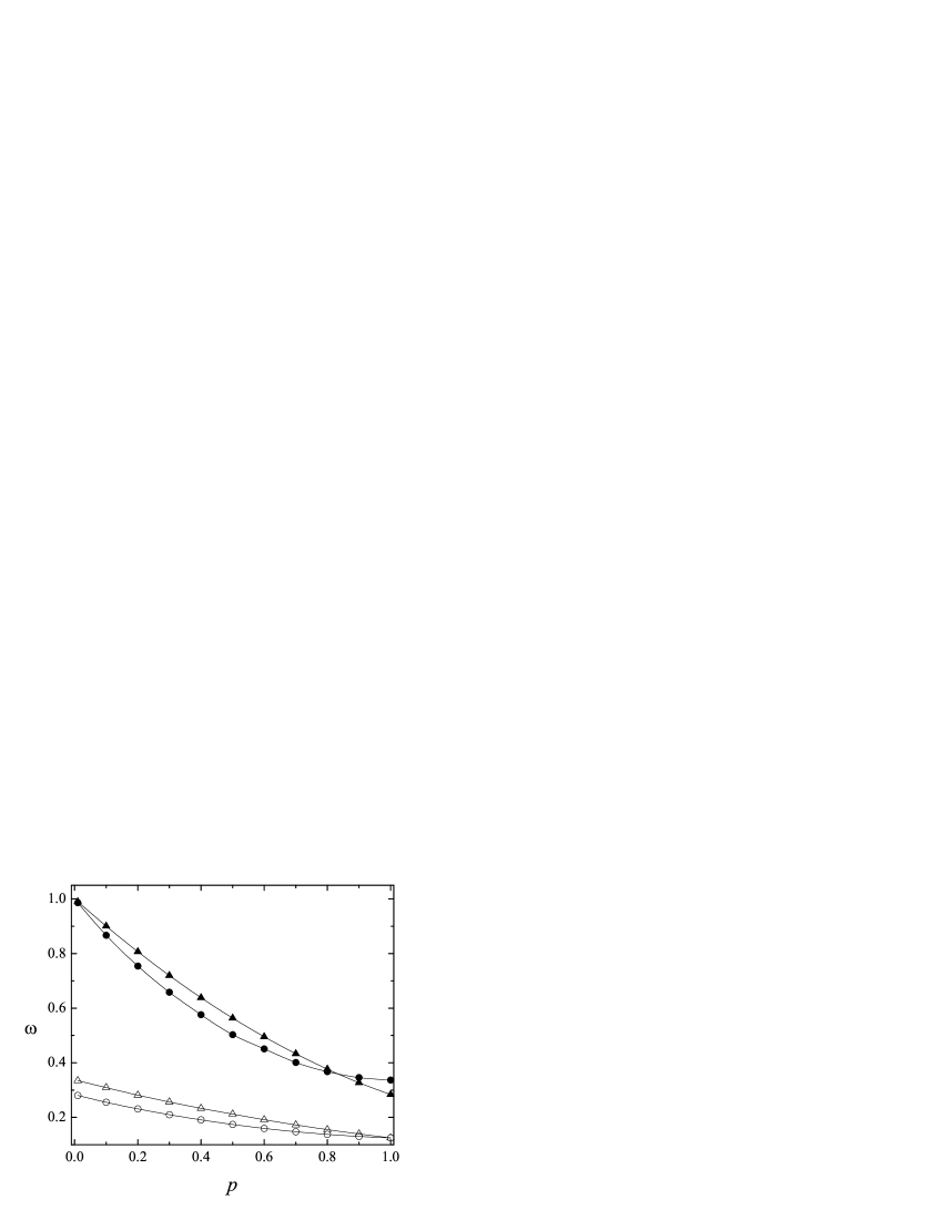
Figure 2: The average overlap ${\omega}$, as a function of $p$, where $p=p_{s}$ (triangles), $p=p_{f}$ (circles), and $p_{d}=0$ in all cases plotted here. Solid symbols indicate that the non-varying $p$ parameter is one, whereas open symbols indicate the non-varying $p$ parameter is zero.

An interesting aspect that leads us to consider diffusion within the system, is the evolution of the size of the cluster of active individuals. For this we have performed several calculations considering an initial active agent located at the center of the system. For several values of $\overline{p}$ and considering the variance of only one $p$ parameter at a time, we have evaluated the mean radius of the growing nucleus. The radius evolves linearly with time and thus the velocity of propagation of the active state $v$, is easily calculated. In Fig. 3, $v$ is depicted as a function of $p$ for each dynamic process. The inset shows $v$ as a function of the mean overlap. Apparent from the figure, the velocity adopts a different behavior for each of the three dynamic processes.

Figure 3: The average velocity of propagation $v$, as a function of $p$, where $p=p_{d}$(squares), $p=p_{s}$ (triangles), and $p=p_{f}$ (circles). In the inset we plot $v$ as a function of ${\omega}$

In conjunction with analytic calculations of the diffusive process, we have performed numerical simulations to measure the mean square displacement $\langle x^{2}\rangle$, where $\langle$ $\rangle$ indicates the mean value over individuals and $x$ is the position of a random walker on the $x$ axis. From the analysis of this quantity throughout time, we obtain a value for the diffusion coefficient. Fig. 4 shows this value as a function of each of the three processes defined by $p_{s}$, $p_{d}$, and $p_{f}$. To compare numerical results with the $\alpha$ and $\beta$ values obtained before, we have considered several individuals performing a random walk in the system. Walkers move along the centers of the domains. A given jump is allowed only if superposition between two domains occurs in two successive time steps. The results correspond to networks undergoing the different processes governed by the aforementioned $p$ parameters. The fitting by minimum squares methods gives us the following values: $D_{d}=1.6p_{d}$, $D_{s}=0.27p_{s}$ and $D_{f}=p_{f}$, which are in agreement with previously calculated values.

Figure 4: Diffusion coefficients as functions of $p$, where $p=p_{d}$(squares), $p=p_{s}$ (triangles), and $p=p_{f}$ (circles). Solid lines indicate the analytic calculation over which the numerical results are plotted.

V Disease propagation

The DDN model that we have proposed compares to previously obtained results of disease propagation within Dynamic Small World Networks zan in the following way. We consider a standard model Murray for an infectious disease with three stages: susceptible (S), infectious (I), and refractory (R). Any susceptible individual can become infected with a given probability by an infected individual within the same domain or neighborhood. The infection cycle ends when the element reaches the refractory state after $\tau$ time steps. The refractory state is a permanent condition and thus the individual cannot be infected again. The algorithm goes as follows. At each step an infected element $i$ is chosen at random. If the time elapsed from the moment $t_{i}$ when it entered the infection cycle up to the current time $t$ is larger than the infection time $\tau$, the element $i$ becomes refractory. Otherwise, one of its neighbors $j$ of $i$ is randomly selected. If $j$ is in the susceptible state, contagion occurs. Element $j$ becomes infected and its infection time $t_{j}=t$ is recorded. If on the other hand, $j$ is already infected or refractory, it preserves its state. Since each time step corresponds to the choice of an infected individual, the update of the time variable depends on the number $N_{I}(t)$ of infected individuals at each step, $t\to t+1/N_{I}(t)$. Once there is no change in the number of infected individuals for the duration of time necessary for all infected individuals to transform into the refractory state $\tau$, then activation time has been achieved and the process stops. Here we set $\tau=3$ for the infection time which insures that for intermediate values of the $\overline{p}$ parameters, the disease spreads over a finite fraction of the population. Moreover, we consider an initial condition where there is only one infected element; all the other elements being susceptible. The considered initial condition thus represents an initially localized disease. The infection will remain localized during the initial stages and will propagate according to the behavior of the domains. In Fig. 5 we plot the proportion of total infected individuals $i_{f}$ as it varies with different values of $p$. Two of the $p$ values are maintained fixed while the remaining one varies between zero and one.

Figure 5: The fraction of infected individuals with respect to the total population $i_{f}$, as a function of $p$, with $p=p_{d}$(squares), $p=p_{s}$ (triangles), and $p=p_{f}$ (circles)

In comparison with the results obtained in zan , we find that the threshold values of $p$ for disease propagation are of the same order. The sharp transition from the non-propagative regime to the propagative one as a function of the structure of the network is one of the most interesting aspects presented by epidemiological models on networks. The maximum proportion of infected individuals shows that a fraction of individuals remain not infected. Similar values of final infected individuals have been obtained in zan . The non-monotonic behavior of this quantity has also been observed in other epidemiological models based on Small World Networks kup . A possible explanation for the decrease of infection for large values of $p_{s}$ involves the fact that in the DDN system, there is a bias towards decreasing the size of a domain. A high level of dynamics will temporally isolate infected individuals. It is because of this limitation of the model that the infection cannot propagate as efficiently for large $p_{s}$ and a smaller number of infected individuals is detected.

VI Conclusions

If we aim to compare the system presented here with previous work on dynamic Small Worlds, we should limit this comparison to cases when shortcuts only to relatively close neighbors are considered. This restriction is due to the fact that in the present model, new links can only be established with nodes occupying neighbor domains. An interesting aspect despite these limitations is that we still observe some of the features found in dynamic SWN models without such restrictions. In the first part we have studied the behavior of the mean persistence time ${\tau}$, which is similar to the SWN path length, and mean neighborhood overlap ${\omega}$, analogous to the SWN clusterization. Though no analysis of how the domain size scales with these quantities was done, the qualitative similarities ought to be noted. That is, there exists a region in the $p$ parameter space when the system displays a mixture of the two limiting cases, relatively high overlap and relatively low activation time. The value of ${\omega}$ can be analytically obtained for some limiting cases. Further, we have studied the underlying diffusive process occurring on the network. A diffusion coefficient was numerically as well as analytically calculated for the three dynamic processes, $p_{s}$, $p_{f}$, and $p_{d}$ and demonstrated the diffusive contribution of each. As a final application and point of comparison with previous work, we analyze the propagation of an infection. For small $p$ values, an initial infection can not propagate. At a given $p$ value, propagation is possible and grows rapidly to a maximum infected fraction of the entire population as $p$ increases. The threshold values are similar to those previously observed for a dynamic SWN. In this case, we show that despite the fact that there is a transition around the same value of $p$, the behavior of the system strongly depends on which dynamic domain process governs the dynamics of the system.

VII Acknowledgements

M.B. would like to thank the OAS for partial support.

References

- (1) S. Milgram, Psychol. Today 2, 60-67 (1967)
- (2) D. J. Watts and S. H. Strogatz, Nature 393,440–442 (1998).
- (3) D. J. Watts, Small Worlds (Princeton University Press, 1999).
- (4) L. A. N. Amaral, A. Scala, M. Barthélemy and H. E. Stanley, Proc. Natl. Acad. Sci. U.S.A. 97, 11149 (2000).
- (5) S.H. Strogatz, Nature 410, 268, (2001)
- (6) R. Albert and A.L. Barabási, Phys. Rev. Lett. 85, 5234 (2000)
- (7) S.C.Manrubia ,J.Delgado and B.Luque, Europhys.Lett.,53,693(2001).
- (8) M. Cáceres, Elementos de estadística de no equilibrio y sus aplicacones al transporte en medios desordenados (Revert , 2003).
- (9) D. Zanette, Phys. Rev. E 65, 041908 (2002).
- (10) J. D. Murray, Mathematical Biology (Springer,Berlin, 1993).
- (11) D. Zanette and M. Kuperman, Physica A 309, 445 (2002).