Stabilization of a (3+1)D soliton in a Kerr medium by a rapidly oscillating dispersion coefficient

Abstract

Using the numerical solution of the nonlinear Schrödinger equation and a variational method it is shown that (3+1)-dimensional spatiotemporal optical solitons can be stabilized by a rapidly oscillating dispersion coefficient in a Kerr medium with cubic nonlinearity. This has immediate consequence in generating dispersion-managed robust optical soliton in communication as well as possible stabilized Bose-Einstein condensates in periodic optical-lattice potential via an effective-mass formulation. We also critically compare the present stabilization with that obtained by a rapid sinusoidal oscillation of the Kerr nonlinearity parameter.

I Introduction

After the prediction of self-trapping st of an optical beam in a nonlinear medium resulting in an optical soliton 1 , there have been many theoretical and experimental studies to stabilize such a soliton under different conditions of nonlinearity and dispersion. A bright soliton in (1+1) dimension (D) in Kerr medium (cubic nonlinearity) is unconditionally stable for positive or self-focusing (SF) nonlinearity in the nonlinear Schrödinger equation (NLS) 1 . However, in (2+1)D and (3+1)D, in homogeneous bulk Kerr medium one cannot have an unconditionally stable soliton-like beam 1 . (If the nonlinearity is negative or self-defocusing (SDF), any initially created soliton always spreads out 1 .) If the nonlinearity is positive or of SF type, any initially created highly localized soliton is unstable in both (2+1)D and (3+1)D 1 . Such a confined wave packet in (3+1)D is often called a light bullet and represents the extension of a self-trapped optical beam into the temporal domain 1 . The generation of a light bullet is of vital importance in soliton-based communication systems. On the experimental front strong stabilization of (2+1)D discrete vortex solitons in a SF nonlinear medium have been observed in optically induced photonic lattices yyy . Such solitons, however, can only be modeled by a more complicated nonlinearity in the NLS in contrast to the simple cubic Kerr nonlinearity considered in this paper.

Recently, through a numerical simulation as well as a variational calculation based on the NLS it has been shown that a soliton in (2+1)D ber ; mal can be stabilized in a layered medium if a variable Kerr nonlinearity coefficient is used in different layers mal ; ber . A weak modulation of the nonlinearity coefficient along the propagation direction leads to a reasonable stabilization in (2+1)D ber . A much better stabilization results if the Kerr coefficient is a layered medium is allowed to vary rapidly between successive SDF and SF type nonlinearities, i.e., between positive and negative values mal .

However, in recent years optical soliton formed by a controlled variation of dispersion coefficient (dispersion-managed optical soliton) in a Kerr medium has been of general interest in communication A . A dispersion-managed soliton allows robust propagation of pulses and is favored over normal solitons. The recent stabilized optical beam in a nonlinear waveguide array in (1+1)D T , called diffraction managed soliton, is quite similar to the present dispersion-managed optical soliton. That problem was described T by the one dimensional NLS with a periodic dispersion coefficient. Such a periodic variation of the dispersion coefficient leads to a greater stability of the soliton during propagation in (1+1)D T . More recently, Abdullaev et al abdulla have shown by a variational and numerical solution of the NLS that by employing a rapidly varying dispersion coefficient it is possible to stabilize an optical soliton in (2+1)D over large propagation distances.

The possibility of the stabilization of an optical soliton in (2+1)D by dispersion management abdulla and Kerr singularity management abdul ; new ; ueda as well as in (3+1)D by Kerr singularity management unp1 ; unp2 in SF medium has led us to investigate the possibility of the stabilization of an optical soliton in (3+1)D by dispersion management. However, some of these studies were concerned with the stabilization of Bose-Einstein condensates abdul ; ueda ; unp1 using the nonlinear Gross-Pitaevskii equation rmp which is very similar to the NLS structurally. The extension of the problem of stabilization of optical soliton from lower to higher dimensions, e.g. from (1+1)D to (3+1)D, is of great interest in the actual three-dimensional world. It is also more challenging due to the possibility of violent collapse in SF medium in higher dimensions 1 .

We begin the present study with a time-dependent variational solution of the NLS with a rapidly oscillating dispersion coefficient in (3+1)D. The variational method leads to a set of coupled differential equations for the soliton width and chirp parameters, which is solved numerically by the fourth-order Adams-Bashforth method koo . The variational solution illustrates that a (3+1)D light bullet can be stabilized over a large propagation distance in a Kerr SF medium with a rapidly oscillating dispersion coefficient for beam power above a critical value. Next we turn to a complete numerical solution of the partial differential NLS by the Crank-Nicholson method koo2 . The complete numerical solution demonstrates the stabilization of a light bullet over large propagation distance by dispersion management in (3+1)D SF Kerr medium.

We also compare the present stabilization of a light bullet by dispersion management with the stabilization obtained by applying an oscillating Kerr nonlinearity as suggested in Ref. unp2 . We find that both schemes leads to comparable stabilization of a light bullet over a large propagation distance of few thousand units.

Although, the present work is of primary interest in the generation of robust optical solitons, it is also of interest from a mathematical point of view in nonlinear physics in the stabilization of a soliton in three dimensions. Moreover, this investigation has interesting implication in the study of Bose-Einstein condensates. The quantum nonlinear equation governing the evolution of the condensate, known as the Gross-Pitaevskii equation rmp , is identical with the (classical) NLS 1 , for the evolution of optical soliton, although the interpretation of the different variables of these two equations is different. In recent years there has been experimental EX and theoretical TH studies of Bose-Einstein condensates in periodic optical-lattice potentials generated by a standing-wave laser beam. By an effective-mass description, the Gross-Pitaevskii equation for the condensate in a periodic optical-lattice potential can be reduced to a dispersion-managed NLS, where the effective mass could be positive or negative eff . There has already been experimental application of such dispersion management to Bose-Einstein condensates ex . The effective mass can be varied by changing the parameters of the periodic potential abdulla . Once a controlled variation of the effective mass would be possible, it might be possible to stabilize a Bose-Einstein condensate in this fashion.

In Sec. II we present a variational study of the problem and demonstrate the possible stabilization of a light bullet in (3+1)D. In Sec. III we present a complete numerical study based on the NLS to study in detail the stabilization of a dispersion-managed light bullet. We also compare the present stabilization with that by nonlinearity management as in Ref. unp2 . Finally, in Sec. IV we give the concluding remarks.

II Variational Calculation

For anomalous dispersion, the NLS can be written as 1

$$\biggr{[}i\frac{\partial}{\partial z}+\frac{\gamma(z)}{2}\nabla_{\bf r}^{2}+|{u({\bf r},z)}|^{2}\biggr{]}u({\bf r},z)=0,$$ (1)

where in (3+1)D the three dimensional vector ${\bf r}\equiv(x,y,t)$ has space components $x$ and $y$ and time component $t$, and $z$ is the direction of propagation. The Laplacian operator $\nabla_{\bf r}^{2}$ acts on the variables $x$, $y$, and $t$. The dispersion coefficient $\gamma(z)$ in a Kerr medium is taken to be rapidly oscillating and can have successive positive and negative values. The normalization condition is $\int d{\bf r}|u({\bf r},z)|^{2}=P$, where $P$ is the power of the optical beam st ; mal .

For a spherically symmetric soliton in (3+1)D, $u({\bf r},z)=U(r,z)$. Then the radial part of the NLS (1) becomes 1

$$\biggr{[}i\frac{\partial}{\partial z}+\frac{\gamma(z)}{2}\frac{\partial^{2}}{\partial r^{2}}+\frac{\gamma(z)}{r}\frac{\partial}{\partial r}+\left|{U({r},z)}\right|^{2}\biggr{]}U({r},z)=0.$$ (2)

For stabilization of the soliton, we shall employ the following oscillating dispersion coefficient: $\gamma(z)=[1+g_{1}\sin(\omega z)]$, where frequency $\omega$ is large. In this paper we consider variational and numerical solutions of Eq. (2) to illustrate the stabilization of a (3+1)D light bullet.

Recently, it was suggested unp2 that a rapid variation of the Kerr nonlinearity parameter also stabilizes a soliton. In this study we critically compare these two ways of stabilization. For that purpose we consider

$$\biggr{[}i\frac{\partial}{\partial z}+\frac{1}{2}\frac{\partial^{2}}{\partial r^{2}}+\frac{1}{r}\frac{\partial}{\partial r}+n(z)\left|{U({r},z)}\right|^{2}\biggr{]}U({r},z)=0,$$ (3)

where the nonlinearity parameter will be taken to be rapidly varying for stabilizing the soliton. In Ref. unp2 $n(z)$ was taken to be rapidly jumping between positive and negative values and a small propagation distance $z$ was considered for stabilization. In the present study a sinusoidal variation of $n(z)$ is considered over a much larger propagation distance. For stabilization we consider $n(z)=[1-g_{2}\sin(\omega z)]$ in this paper, where the second term on the right is rapidly oscillating for a large $\omega$ and where $g_{2}$ is a constant.

First we consider the variational approach with the following trial Gaussian wave function for the solution of Eq. (2) ueda ; abdul ; unp2 ; 1

$$U(r,z)=N(z)\exp\left[-\frac{r^{2}}{2R^{2}(z)}+\frac{i}{2}{b(z)}r^{2}+i\alpha(z)\right],$$ (4)

where $N(z)$, $R(z)$, $b(z)$, and $\alpha(z)$ are the soliton’s amplitude, width, chirp, and phase, respectively. In Eq. (4) $N(z)={P^{1/2}}/{[\pi^{3/4}R^{3/2}(z)]}$. The trial function (4) satisfies (a) the normalization condition st ; mal as well as the boundary conditions (b) $U(r,z)\to$ constant as $r\to 0$ and (c) $|U(r,z)|$ decays exponentially as $r\to\infty$ mal .

The Lagrangian density for generating Eq. (2) is abdul ; unp2

$${\cal L}(U)=\frac{i}{2}\left(\frac{\partial U}{\partial z}U^{*}-\frac{\partial U^{*}}{\partial z}U\right)-\frac{\gamma}{2}\left|\frac{\partial U}{\partial r}\right|^{2}+\frac{|U|^{4}}{2},$$ (5)

where the functional dependence of the quantities on $r$ and $z$ is suppressed. The trial function (4) is substituted in the Lagrangian density and the effective Lagrangian is calculated by integrating the Lagrangian density: $L_{\mbox{eff}}=\int{\cal L}(U)d\bf r.$ With $U$ given by Eq. (4) the effective Lagrangian is

$$L_{\mbox{eff}} = \frac{1}{2}\pi^{3/2}N^{2}(z)R^{3}(z)\biggr{[}-\frac{3}{2}\dot{b}(z)R^{2}(z)-2\dot{\alpha}(z)$$ (6)

$$+ \frac{N^{2}(z)}{2\sqrt{2}}-\frac{3}{2}\frac{\gamma(z)}{R^{2}(z)}-\frac{3}{2}R^{2}(z)b^{2}(z)\gamma(z)\biggr{]},$$

where the overhead dot denotes derivative with respect to $z$. The standard Euler-Lagrange equations for $N(z)$, $R(z)$, $b(z)$, and $\alpha(z)$ are mal ; abdul ; ueda given by

$$\frac{d}{dz}\frac{\partial L_{\mbox{eff}}}{\partial\dot{\beta}}=\frac{\partial L_{\mbox{eff}}}{\partial\beta},$$ (7)

where $\beta$ stands for $N(z)$, $R(z)$, $b(z)$, or $\alpha(z)$. The Euler-Lagrange equation for $\alpha(z)$ gives the normalization:

$$\pi^{3/2}N^{2}R^{3}=P.$$ (8)

The Euler-Lagrange equations for $R(z)$ and $N(z)$ are given by

$$5\dot{b}+\frac{4\dot{\alpha}}{R^{2}}+\frac{\gamma}{R^{4}}+5b^{2}\gamma=\frac{N^{2}}{\sqrt{2}R^{2}}$$ (9)

$$3\dot{b}+\frac{4\dot{\alpha}}{R^{2}}+\frac{3\gamma}{R^{4}}+3b^{2}\gamma=\frac{2N^{2}}{\sqrt{2}R^{2}},$$ (10)

where the $z$ dependence of the variables is suppressed. The Euler-Lagrange equation for $b(z)$ is

$$\dot{R}(z)=R(z)b(z)\gamma(z).$$ (11)

Equations (9) and (10) leads to the following rate of variation of $b(z)$:

$$\dot{b}(z)=\frac{\gamma(z)}{R^{4}(z)}-b^{2}(z)\gamma(z)-\frac{P}{2\sqrt{2\pi^{3}}}\frac{1}{R^{5}(z)}.$$ (12)

Now defining the new variable $\kappa(z)=b(z)R(z)$, Eqs. (11) and (12) can be rewritten as

$$\dot{R}(z) = \gamma(z)\kappa(z)$$ (13)

$$\dot{\kappa}(z) = \frac{\gamma(z)}{R^{3}(z)}-\frac{P}{2\sqrt{2\pi^{3}}}\frac{1}{R^{4}(z)}.$$ (14)

Equations (13) and (14) are the variational equations of motion for $R(z)$ and $\kappa(z).$ Here we consider the stability condition of optical solitons described variationally by these equations for $\gamma(z)=[1+g_{1}\sin(\omega z)]$, where the second term is rapidly varying (large $\omega$) with zero mean value. However, this set of coupled differential equations cannot be solved analytically and we resort to their numerical solution using the four-step Adams-Bashforth method koo . For a large $\omega$ and $P$, and $g_{1}\geq 2$ stabilization of the soliton is always possible provided that the initial values of $R(z)$ and $\kappa(z)$ are appropriately chosen. The soliton can also be stabilized by employing a periodically oscillating Kerr nonlinearity. However, in that case the coupled set of differential equations for width $R(z)$ and chirp $b(z)$ was simpler and could be studied analytically to establish stabilization of the system unp2 .

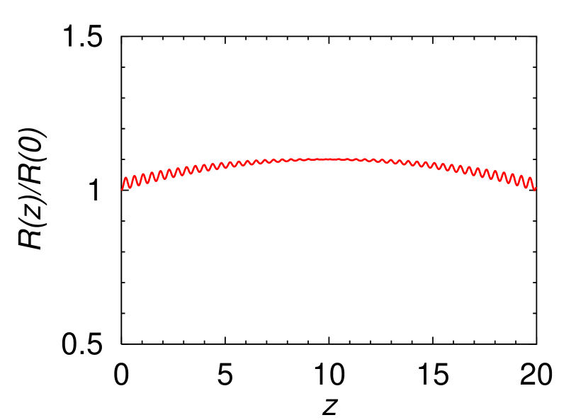
Figure 1: The width of the soliton $R(z)/R(0)$ vs. propagation distance $z$ from the numerical solution of the coupled set of equations (13) and (14), with $\gamma(z)=[1+g_{1}\sin(\omega z)]$ for $P=500,g_{1}=4,\omega=15,R(0)=6$ and $\kappa(0)=0.14$.

In Fig. 1 we exhibit the numerical results for the width $R(z)$ obtained from the solution of the variational equations (13) and (14). In the present calculation we take $\omega=15$, $g_{1}=4$, $P=500$, and $R(z=0)=6$ If the initial value of $b(z)$ is chosen appropriately, stabilization of the system can be obtained. For these set of parameters, stabilization was obtained for $b(z=0)=0.14$, and we show the result in Fig. 1, where we plot $R(z)/R(0)$ vs. $z$. The width $R(z)$ is found to to remain stable for a range of values of $z$. Small oscillations in Fig. 1 sustain the soliton for a large propagation distance $z$. The numerical values for $g_{1}$ and $\omega$ are taken as examples, otherwise they do not have great consequence on the result so long as $\omega$ is large corresponding to rapid oscillation. There is no upper limit for $P$ and stabilization seems possible for an arbitrarily large $P$. For larger $P$ the stabilization is more sustained and consequently, it is easier to stabilize a soliton. However, SF nonlinearity is essential for the stabilization and stabilization is only possible for power $P$ above a critical value.

The sinusoidal variation of the dispersion coefficient as considered above in the variational study only simplifies the algebra and is by no means necessary for stabilization of solitons. Any rapid periodic oscillation of the dispersion coefficient was also found to stabilize the soliton. The same was found to be true in the stabilization of a soliton by Kerr-singularity management in (3+1)D unp1 ; unp2 .

III Numerical Result

Motivated by the approximate variational study above, now we solve Eqs. (2) and (3) numerically using a split-step iteration method employing the Crank-Nicholson discretization scheme koo2 ; 11 . The $z$-iteration is started with the known solution of some auxiliary equation with zero nonlinearity. The auxiliary equation with known Gaussian solution is obtained by adding a harmonic oscillator potential $r^{2}$ to Eqs. (2) and (3) and setting the nonlinear term to zero, e.g.,

$$\biggr{[}i\frac{\partial}{\partial z}+\frac{1}{2}\frac{\partial^{2}}{\partial r^{2}}+\frac{1}{r}\frac{\partial}{\partial r}+\frac{d(z)r^{2}}{4}\biggr{]}U({r},z)=0.$$ (15)

In Eq. (15) we have introduced a strength parameter $d(z)$ with the radial trap. Normally, $d(z)=1$; when the radial trap is switched off $d(z)$ will be reduced to zero. Asymptotically decaying real boundary condition for $U(r,z)$ is used throughout this calculation.

When the radial trap is reduced to zero the wave function extends to a large value of $r$. Hence to obtain a converged result a large value of $r$ is to be considered in the Crank-Nicholson discretization scheme. In the present calculation we employ an $r$-step of 0.1 with 40 000 grid points spanning an $r$-value up to 4000 and a $z$-step of 0.001. In the course of $z$-iteration a positive SF Kerr nonlinearity with appropriate power $P$ is switched on slowly and the harmonic trap is also switched off slowly. If the nonlinearity is increased rapidly the system collapses. The tendency to collapse or expand to infinity must be avoided to obtain a stabilized soliton. Although, for the sake of convenience we applied a harmonic trap in the beginning of our simulation, which is removed later with the increase of nonlinearity, this restriction is by no means necessary for stabilizing a soliton.

First we consider the numerical solution of Eq. (2) to create the desired soliton. After switching off the harmonic trap and introducing the final power $P$, the oscillating dispersion coefficient $\gamma(z)=[1+g_{1}\sin(\omega z)]$ is introduced. A stabilization of the final solution could be obtained for a large $\omega$ and $P$. If the SF power after switching off the harmonic trap is large compared to the spatiotemporal size of the beam the system becomes highly attractive in the final stage and it eventually collapses. If the final power after switching off the harmonic trap is small for its size the system becomes weakly attractive in the final stage and it expands to infinity. The final power has to have an appropriate value consistent with the size, for final stabilization.

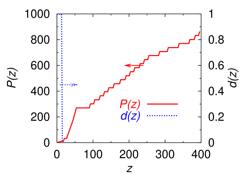
Figure 2: (Color online) Variation of power $P(z)$ and strength $d(z)$ of radial trap in the initial stage of stabilization until the radial trap removed and the final power $P=868.4$ attained at $z=400$.

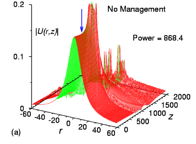
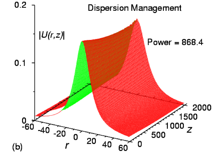
Figure 3: (Color online) (a) The solitonic wave function $|U(r,z)|$ vs. $r$ and $z$ of a freely propagating light bullet of power $P=868.4$, the arrow at $z=300$ shows the beginning of collapse with $|U(r=0,z)|$ starting to diverge; (b) The solitonic wave function $|U(r,z)|$ of Eq. (2) vs. $r$ and $z$ of the light bullet of (a) stabilized by dispersion management $\gamma(z)=[1+4\sin(5\pi z)]$ applied for all $z>0$; (c) The solitonic wave function $|U(r,z)|$ of Eq. (3) vs. $r$ and $z$ of the light bullet of (a) stabilized by Kerr nonlinearity management $n(z)=[1-4\sin(5\pi z)]$ applied for all $z>0$.

Starting from Eq. (15) the soliton can be created with a wide range of variation of power $P(z)$ and strength $d(z)$. In Fig. 2 we show the actual variation of $P(z)$ and $d(z)$ of the radial trap in Eq. (15). A stabilized soliton can be obtained for different variations of $P(z)$ and $d(z)$ and the variation in Fig. 2 are by no means unique and are to be considered as a possible variation. By switching off the harmonic trap linearly for $13<z<15$ and increasing the nonlinearity for $0<z<400$, an almost stationary light bullet is prepared. One interesting feature of Fig. 2 is that we could not find a linear variation of $P(z)$ over the whole range to obtain the final soliton. A linear variation usually led to collapse or expansion to infinity of the final soliton. A fine-tuning of the power was needed for obtaining the quasi-stationary soliton with the kinetic pressure almost balancing the nonlinear attraction. This fine-tuning led to the final fractional power $P=868.4$. A quasi-stationary soliton, rather than a rapidly expanding or collapsing soliton, was ideal for stabilization. Although the final power $P=868.4$ is used in this study, stabilization can be obtained for any $P$ greater than a critical value.

In the preparation of the soliton in Fig. 2 no oscillating dispersion coefficient has been used. The oscillating dispersion coefficient has been applied later. In (2+1)D Saito and Ueda ueda first applied a weak oscillating nonlinearity and then increased its strength in a linear fashion with $z$ iteration. The nonlinearity manipulation of Saito and Ueda ueda is distinct from ours. However, the final result should be independent of how the oscillating dispersion or nonlinearity coefficient is introduced.

The propagation of the free light bullet is studied by a direct numerical solution of the NLS (2). Once it is allowed to propagate in the $z$ direction the light bullet starts to collapse and is destroyed after propagating a distance of about 300 units of $z$ as shown in Fig. 3 (a) where we plot the profile of the freely propagating light bullet $|U(r,z)|$ vs. $r$ and $z$. This means that the nonlinear attraction supersedes the kinetic pressure in this soliton and it collapses eventually.

In the present scheme of stabilization the dispersion coefficient $\gamma(z)=[1+g_{1}\sin(\omega z)]$ oscillates rapidly between positive and negative values. A negative dispersion coefficient $\gamma(z)$ corresponds to collapse and a positive dispersion coefficient corresponds to expansion. In one half of the oscillating cycle the soliton tends to collapse and in the other half it tries to expand. If, in the first semi-cycle of the application of the oscillating dispersion coefficient, $\gamma(z)$ is positive, the slowly collapsing soliton of Fig. 3 (a) will tend to expand in this semi-cycle. In the next semi-cycle, $\gamma(z)$ will be negative and the soliton will tend to collapse. This happens for a positive $g_{1}>1$. If the expansion in the first interval is compensated for by the collapse in the next interval, a stabilization of the system is obtained. However, if $g_{1}$ is negative, in the first semi-cycle of oscillation the slowly collapsing soliton of Fig. 3 (a) will collapse further and a satisfactory stabilization cannot be obtained. For a large $\omega$ the system remains virtually static and the very small oscillations arising from collapse and expansion remain unperceptible.

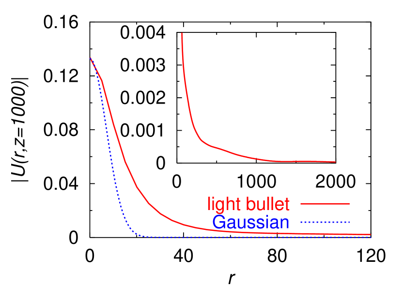
Figure 4: (Color online) The wave function $|U(r,z=1000)|$ of the stabilized light bullet of Figs. 3 (b) and (c) vs. $r$. For comparison the Gaussian ($\sim\exp(-r^{2}/100)$) is also shown.

Next using Eq. (2) we illustrate the possible stabilization of the (3+1)D soliton of power $P=868.4$ of Fig. 3 (a) by the application of the oscillating dispersion coefficient $\gamma(z)=[1+g_{1}\sin(\omega z)]$ with $g_{1}=4$ and $\omega=5\pi$ for $z>0$. The profile of the dispersion-managed light bullet $|U(r,z)|$ vs. $r$ and $z$ is plotted in Fig. 3 (b). It is realized that after the application of dispersion management the soliton remains stable for a large propagation distance $z$. This shows clearly the effect of the oscillating dispersion coefficient on stabilization. The dispersion management of the type considered in Fig. 3 (b) can prolong the life of the soliton significantly. In Fig. 3 (b) the profile of the solitonic wave function over the large interval of $z$ clearly shows the quality of stabilization. The stabilization seems to be good and can be continued for longer intervals of $z$ by considering a soliton of larger power.

Finally, using Eq. (3) we consider the stabilization of the above soliton of power $P=868.4$ by the application of an oscillating Kerr nonlinearity $n(z)=[1-g_{2}\sin(\omega z)]$ with $g_{2}=4$ and $\omega=5\pi$ for $z>0$. In this case for $g_{2}>1$, the Kerr nonlinearity coefficient $n(z)$ is negative in the first semi-cycle of the oscillating Kerr coefficient. This will correspond to an expansion of the soliton, so that the collapsing tendency of the soliton of Fig. 3 (a) could be stopped and a stabilization of the soliton could be obtained. The profile of the stabilized light bullet by nonlinearity management is plotted in Fig. 3 (c). It is found that the oscillating Kerr nonlinearity can stabilize the light bullet for a large propagation distance and enhance the life of the soliton significantly. The quality of stabilization is comparable to that obtained by dispersion management. In both schemes the light bullet can remain stable for few thousands units of $z$. In Figs. 3 we illustrate this stabilization for $z$ up to 2000. The stabilization obtained in (2+1)D by similar dispersion abdulla and nonlinearity mal ; abdul ; new ; ueda managements was over a much smaller interval of $z$ ($<100$).

The final solitonic wave function $|U(r,z)|$ extends to very large values of $r$. It has a sharp peak for small $r$, reminiscent of strong binding, and a large extention in $r$, typical of weak binding. We illustrate these features in Fig. 4 where we plot $|U(r,z=1000)|$ of a light bullet vs. $r$ for dispersion or nonlinearity managements of Figs. 3 (b) and (c). The curves for dispersion and nonlinearity managements are identical with each other and a single curve is shown. The long tail of the stabilized light bullet is shown in inset. For comparison a Gaussian ($\sim\exp(-r^{2}/100)$) is also shown.

For both dispersion and nonlinearity managements we found that the stabilization can only be obtained for beams with power larger than a critical value. However, we could not obtain a precise value of this critical power numerically. In Ref. unp2 we obtained a variational estimate of this critical power ($\sim 40$) for nonlinearity management. We could not obtain such an estimate for dispersion management. Numerically, we found that it was easier to obtain stabilization of beams with power much larger than the critical value.

IV Conclusion

In conclusion, after a variational and numerical study of the NLS we find that it is possible to stabilize a spatiotemporal light bullet by employing a rapidly oscillating dispersion coefficient. We find that the nature of this stabilization is similar to that obtained by a rapid variation of the Kerr-nonlinearity parameter. In both cases stabilization is possible in a SF Kerr medium for optical beams with power $P$ larger than a critical value. However, there is no upper limit of $P$ for stabilization. A larger value of $P$ is preferred for stabilization. The stabilization of the light bullet by dispersion and Kerr nonsingularity management unp2 should find experimental application in optics and Bose-Einstein condensation. Such a dispersion- and nonsingularity-managed optical soliton can propagate large distances with a minimum of distortion and is to be preferred over normal solitons in optical communication.

- (1) R. Y. Chiao, E. Garmire, and C. H. Townes, Phys. Rev. Lett. 13, 479 (1964).
- (2) A. Hasegawa and F. Tappert, Appl. Phys. Lett. 23, 171 (1973); 23, 142 (1973); V. E. Zakharov and A. B. Shabat Sov. Phys. JETP 34, 62 (1972); 37, 823 (1973).
- (3) Y. S. Kivshar and G. P. Agrawal, Optical Solitons - From Fibers to Photonic Crystals, (Academic Press, San Diego, 2003).
- (4) D. N. Neshev, T. J. Alexander, E. A. Ostrovskaya, and Y. S. Kivshar, H. Martin, I. Makasyuk, and Z. Chen, Phys. Rev. Lett. 92, 123903 (2004).
- (5) L. Bergé, V. K. Mezentsev, J. J. Rasmussen, P. L. Christiansen, and Yu. B. Gaididei, Opt. Lett. 25, 1037 (2000).
- (6) I. Towers and B. A. Malomed, J. Opt. Soc. Am. B 19, 537 (2002).
- (7) N. J. Smith, F. M. Knox, N. J. Doran, K. J. Blow, and I. Bennion, Electron. Lett. 32, 54 (1996); I. Gabitov and S. K.Turitsyn, Opt. Lett. 21, 327 (1996).
- (8) M. J. Ablowitz and Z. H. Musslimani, Phys. Rev. Lett. 87, 254102 (2001); Phys. Rev. E 65, 056618 (2002).
- (9) F. K. Abdullaev, B. B. Baizakov, and M. Salerno, Phys. Rev. E 68, 066605 (2003).
- (10) F. K. Abdullaev, J. G. Caputo, R. A. Kraenkel, and B. A. Malomed, Phys. Rev. A 67, 013605 (2003); J. Low Temp. Phys. 134, 671 (2004).
- (11) G. D. Montesinos, V. M. Perez-Garcia, and P. J. Torres, Physica D 191, 193 (2004); G. D. Montesinos, V. M. Perez-Garcia, and H. Michinel, Phys. Rev. Lett. 92, 133901 (2004).
- (12) H. Saito and M. Ueda, Phys. Rev. Lett. 90, 040403 (2003).
- (13) S. K. Adhikari, Phys. Rev. A 69, 063613 (2004).
- (14) S. K. Adhikari, Phys. Rev. E 70, 036608 (2004).
- (15) F. Dalfovo, S. Giorgini, L. P. Pitaevskii, and S. Stringari, Rev. Mod. Phys. 71, 463 (1999).
- (16) S. E. Koonin, Computational Physics, (Benjamin/Cummings, Menlo Park, 1986), pp 27.
- (17) Ref. koo , Ch. 7.
- (18) F. S. Cataliotti, S. Burger, C. Fort, P. Maddaloni, F. Minardi, A. Trombettoni, A. Smerzi, and M. Inguscio, Science 293, 843 (2001); M. Greiner, O. Mandel, T. Esslinger, T. W. Hansch, and I. Bloch, Nature 415, 6867 (2002).
- (19) S. K. Adhikari, Eur. Phys. J. D 25, 161 (2003); S. K. Adhikari and P. Muruganandam, Phys. Lett. A 310, 229 (2003).
- (20) H. Pu, L. O. Baksmaty, W. Zhang, N. P. Bigelow, and P. Meystre, Phys. Rev. A 67, 043605 (2003); H. Sakaguchi and B. A. Malomed, J. Phys. B 37, 1443 (2004).
- (21) B. Eiermann, P. Treutlein, Th. Anker, M. Albiez, M. Taglieber, K.-P. Marzlin, and M. K. Oberthaler, Phys. Rev. Lett. 91, 060402 (2003).
- (22) S. K. Adhikari and P. Muruganandam, J. Phys. B 35, 2831 (2002); 36, 409 (2003); P. Muruganandam and S. K. Adhikari, ibid. 36, 2501 (2003).