Exact solutions of the Saturable Discrete Nonlinear Schrödinger Equation

Abstract

Exact solutions to a nonlinear Schrödinger lattice with a saturable nonlinearity are reported. For finite lattices we find two different standing-wave-like solutions, and for an infinite lattice we find a localized soliton-like solution. The existence requirements and stability of these solutions are discussed, and we find that our solutions are linearly stable in most cases. We also show that the effective Peierls-Nabarro barrier potential is nonzero thereby indicating that this discrete model is quite likely nonintegrable.

The discrete nonlinear Schrödinger (DNLS) equation occurs ubiquitously KRB throughout modern science. Most notable is the role it plays in understanding the propagation of electromagnetic waves in glass fibers and other optical waveguides OP . More recently it has been applied to describe Bose-Einstein condensates in optical lattices ST . Here we are concerned with the DNLS equation with a saturable nonlinearity

$$i\dot{\psi}_{n}+(\psi_{n+1}+\psi_{n-1}-2\psi_{n})+\frac{\nu|\psi_{n}|^{2}}{1+\mu|\psi_{n}|^{2}}\psi_{n}=0,$$ (1)

which is an established model for optical pulse propagation in various doped fibers fibers . In Eq. (1), $\psi_{n}$ is a complex valued “wave function” at site $n$, while $\nu$ and $\mu$ are real parameters. This equation represents a Hamiltonian system with:

$${\cal H}=\sum_{n=1}^{N}\left[|\psi_{n}-\psi_{n+1}|^{2}-\frac{\nu}{\mu}|\psi_{n}|^{2}+\frac{\nu}{\mu^{2}}\ln\left(1+\mu|\psi_{n}|^{2}\right)\right],$$ (2)

so that Eq. (1) is given by $i\dot{\psi}_{n}=\frac{\partial{\cal H}}{\partial\psi_{n}^{*}}$. The dynamics of Eq. (1) conserve, in addition to the Hamiltonian ${\cal H}$, the power ${\cal P}$

$${\cal P}=\sum_{n=1}^{N}|\psi_{n}|^{2}.$$ (3)

In the above equations $N$ is the number of lattice sites in the system. We note that a transformation $\sqrt{\nu}\psi_{n}\rightarrow\psi_{n}$ will replace $\nu$ by 1 and $\mu$ by $\frac{\mu}{\nu}$ in the above equations. Note also that Eq. (1) is invariant under the transformation $\psi_{n}\rightarrow\exp(i\delta)\psi_{n}$ where $\delta$ represents an abitrary phase.

For given system parameters $\nu$ and $\mu$ it can be shown, using recently derived Khare local and cyclic identities for Jacobi elliptic functions stegun , that Eq. (1) has two (Case I and Case II) different temporally and spatially periodic solutions. Both solutions possess the temporal frequency

$$\omega=2\left(1-\frac{\nu}{2\mu}\right).$$ (4)

Using standard notation stegun for the Jacobi elliptic functions of modulus $m$ the solutions can be expressed as

Case I:

$$\psi_{n}^{I}=\frac{1}{\sqrt{\mu}}\frac{\mbox{sn}(\beta,m)}{\mbox{cn}(\beta,m)}\mbox{dn}([n+c]\beta,m)\exp\left(-i[\omega t+\delta]\right),$$ (5)

where the modulus $m$ must be chosen such that

$$\frac{2\mu}{\nu}=\frac{\mbox{cn}^{2}(\beta,m)}{\mbox{dn}(\beta,m)},~{}~{}\beta=\frac{2K(m)}{N_{p}},$$ (6)

and $c$ and $\delta$ are arbitrary constants. We only need to consider c between 0 and $\frac{1}{2}$ (half the lattice spacing). Here $K(m)$ denotes the complete elliptic integral of first kind stegun . While obtaining this solution, use has been made of the local identity

$$\mbox{dn}^{2}(x,m)[\mbox{dn}(x+a,m)+\mbox{dn}(x-a,m)]=-\frac{\mbox{cn}^{2}(a,m)}{\mbox{sn}^{2}(a,m)}[\mbox{dn}(x+a,m)+\mbox{dn}(x-a,m)]+2\frac{\mbox{dn}(a,m)}{\mbox{sn}^{2}(a,m)}\mbox{dn}(x,m)\,,$$ (7)

derived recently Khare . In fact, given Eq. (1) and this local identity [and similar ones for $\mbox{sn}(x,m)$ and $\mbox{cn}(x,m)$], it was straightforward to obtain the two solutions presented here and the third solution follows simply by taking the limit $m\rightarrow 1$ of these two solutions as shown below.

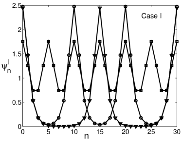
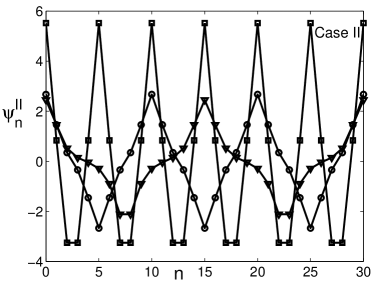
Figure 1: Illustration of the exact solutions of two types. $\nu=1$, $\mu=0.3$, $\omega=-1.33$, and $c=t=\delta=0$. $N_{p}=5$ (squares), $N_{p}=10$ (circles), and $N_{p}=15$ (triangles). Lines are guides to the eye.

Case II:

$$\psi_{n}^{II}=\sqrt{\frac{m}{\mu}}\frac{\mbox{sn}(\beta,m)}{\mbox{dn}(\beta,m)}\mbox{cn}([n+c]\beta,m)\exp\left(-i[\omega t+\delta]\right),$$ (8)

where modulus $m$ now is determined such that

$$\frac{2\mu}{\nu}=\frac{\mbox{dn}^{2}(\beta,m)}{\mbox{cn}(\beta,m)},~{}~{}\beta=\frac{4K(m)}{N_{p}}.$$ (9)

While obtaining this solution, use has been made of the local identity Khare

$$m\mbox{cn}^{2}(x,m)[\mbox{cn}(x+a,m)+\mbox{cn}(x-a,m)]=-\frac{\mbox{dn}^{2}(a,m)}{\mbox{sn}^{2}(a,m)}[\mbox{dn}(x+a,m)+\mbox{dn}(x-a,m)]+2\frac{\mbox{cn}(a,m)}{\mbox{sn}^{2}(a,m)}\mbox{cn}(x,m)\,.$$ (10)

Note that the two solutions, Eqs. (5) and (8), are translationally invariant.

The two solutions $\psi_{n}^{I,II}$ are illustrated in Fig. 1 for $t=\delta=c=0$. In both cases the integer $N_{p}$ denotes the spatial period of the solutions. Both the solutions $\psi_{n}^{I}$ and $\psi_{n}^{II}$ reduce to the same localized solution in the limit $N_{p}\rightarrow\infty$ ($m\rightarrow 1$):

Case III:

$$\psi_{n}^{III}=\frac{1}{\sqrt{\mu}}\frac{\sinh(\beta)}{\cosh([n+c]\beta)}e^{-i[\omega t+\delta]},~{}~{}(N_{p}\rightarrow\infty),$$ (11)

where $\beta$ is now given by

$$\mbox{sech}\beta=\frac{2\mu}{\nu}.$$ (12)

Again the frequency $\omega$ is given by Eq. (4). This solution is noteworthy in that it is very similar in form to the celebrated exact soliton solutions of both the continuum cubic nonlinear Schrödinger equation Drazin and the (integrable) Ablowitz-Ladik lattice scott

There are, as expressed by Eqs. (6), (9), and (12), stringent conditions on the parameters $\mu$ and $\nu$ for which these exact solutions exist. In the cases I and II these limitations are illustrated in Fig. 2, which shows that the solution $\psi_{n}^{I}$ only exists for parameter values below the lower curve (circles). Similarly, the solution $\psi_{n}^{II}$ for periods $N_{p}>4$ only exists below the upper curve (squares). As can be easily seen from Eq. (9) the $\psi_{n}^{II}$ solution does not exist for $N_{p}=4$. However, it does exist for $N_{p}=3$, but only for parameter ratios $\mu/\nu<0$. As a result of the periodic boundary conditions both solutions become meaningless for $N_{p}<3$. The solution $\psi_{n}^{III}$ exists for all parameter values $\nu\geq 2\mu>0$.

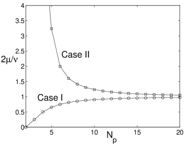
Figure 2: Illustration of parameter values $\mu$, $\nu$, and $N_{p}$ for which the exact solutions are allowed. Case I: $2\mu/\nu$ between 0 and $\cos^{2}\frac{\pi}{N_{p}}$ and $N_{p}\geq 3$. Case II: $2\mu/\nu$ between 0 and $1/\cos^{2}\frac{2\pi}{N_{p}}$ and $N_{p}\geq 3$ except for $N_{p}=4$.

For the $\psi_{n}^{III}$ solution, expressions for both the power Eq. (3) and the Hamiltonian Eq. (2) can be obtained by using exact (Poisson) summation rules Avadh

$${\cal P}^{III}=\frac{2}{\mu}\frac{\mbox{sinh}^{2}(\beta)}{\beta^{2}}\big{[}\beta-2K(m)E(m)+2K^{2}(m)\mbox{dn}^{2}(2K(m)c,m)\big{]},$$ (13)

$${\cal H}^{III}=-\frac{4}{\mu}\mbox{sinh}(\beta)+\left(1-\frac{\nu}{2\mu}\right)\frac{4}{\mu}\frac{\mbox{sinh}^{2}(\beta)}{\beta^{2}}\big{[}\beta-2K(m)E(m)+2K^{2}(m)\mbox{dn}^{2}(2K(m)c,m)\big{]}+\frac{\nu}{\mu^{2}}2\beta.$$ (14)

Here the modulus $m$ must be determined such that

$$\beta=\pi\frac{K(m)}{K(m_{1})},~{}~{}\mbox{sech}\beta=\frac{2\mu}{\nu},$$ (15)

where $m_{1}=1-m$ is the complementary modulus and $E(m)$ denotes the complete elliptic integral of the second kind. For the cases I and II analogous expressions can be obtained and they are given in the Appendix.

In a discrete lattice there is an energy cost associated with moving a localized mode (such as a soliton or a breather) by a half lattice constant. This is called the Peierls-Nabarro (PN) barrier PN ; peyrard . Having obtained the expression for ${\cal H}^{III}$ analytically in a closed form, we can now calculate the energy difference between the solutions when $c=0$ and $c=1/2$, i.e. when the peak of the solution is centered on a lattice site and when it is centered half-way between two adjacent sites, respectively. We find that

$$\Delta E\equiv{\cal H}^{III}(c=0)-{\cal H}^{III}(c=1/2)=-\frac{16m}{\mu\beta^{2}}\sinh^{2}(\beta)\sinh^{2}(\beta/2)K^{2}(m)<0\,,$$ (16)

that is, the energy is lowest when the peak of the solution is centered at the sites. Thus, there is a finite energy barrier (i.e. the height of the effective PN barrier potential) between these two stationary states due to discreteness. If the folklore of nonzero PN barrier being indicative of non-integrability of the discrete nonlinear system is correct, this suggests that quite likely our discrete model is non-integrable unlike the Ablowitz-Ladik model scott .

In order to study the linear stability of the exact solutions $\psi_{n}^{j}$ ($j$ is I, II, or III) we introduce the following expansion

$$\psi_{n}(t)=\psi_{n}^{j}+\delta\psi_{n}(t)e^{-i\omega t},$$ (17)

applied in a frame rotating with frequency $\omega$ of the solution. Substituting into Eq. (1) and retaining only terms linear in the perturbation we get

$$i\delta\dot{\psi}_{n}+\big{(}\delta\psi_{n+1}+\delta\psi_{n-1}-2\delta\psi_{n}\big{)}+\left(\omega+\frac{\nu|\psi_{n}^{j}|^{2}(2+\mu|\psi_{n}^{j}|^{2})}{(1+\mu|\psi_{n}^{j}|^{2})^{2}}\right)\delta\psi_{n}+\frac{\nu|\psi_{n}^{j}|^{2}}{(1+\mu|\psi_{n}^{j}|^{2})^{2}}\delta\psi_{n}^{*}=0.$$ (18)

Continuing by splitting the perturbation $\delta\psi_{n}$ into real parts $\delta u_{n}$ and imaginary parts $\delta v_{n}$ ($\delta\psi_{n}=\delta u_{n}+i\delta v_{n}$) and introducing the two real vectors

$$\delta\mbox{\boldmath$U$}=\{\delta u_{n}\} \delta\mbox{\boldmath$V$}=\{\delta v_{n}\}$$ and (19)

and the two real matrices $\mbox{\boldmath$A$}=\{A_{nm}\}$ and $\mbox{\boldmath$B$}=\{B_{nm}\}$ by defining

$$A_{nm} = \delta_{n,m+1}+\delta_{n,m-1}+\left(\omega-2+\frac{\nu|\psi_{n}^{j}|^{2}(3+\mu|\psi_{n}^{j}|^{2})}{(1+\mu|\psi_{n}^{j}|^{2})^{2}}\right)\delta_{nm},$$ (20)

$$B_{nm} = \delta_{n,m+1}+\delta_{n,m-1}+\left(\omega-2+\frac{\nu|\psi_{n}^{j}|^{2}}{(1+\mu|\psi_{n}^{j}|^{2})}\right)\delta_{nm},$$ (21)

where $m\pm 1$ in the Kronecker $\delta$ means: $m\pm 1~{}mod~{}N$. Then Eq. (18) can be written compactly as

$$-\delta\mbox{\boldmath$\dot{V}$}+\mbox{\boldmath$A$}\delta\mbox{\boldmath$U$}=\mbox{\boldmath$0$}, \delta\mbox{\boldmath$\dot{U}$}+\mbox{\boldmath$B$}\delta\mbox{\boldmath$V$}=\mbox{\boldmath$0$},$$ and (22)

where an overdot denotes time derivative. Combining these first order differential equations we get:

$$\delta\mbox{\boldmath$\ddot{V}$}+\mbox{\boldmath$A$}\mbox{\boldmath$B$}\delta\mbox{\boldmath$V$}=\mbox{\boldmath$0$}, \delta\mbox{\boldmath$\ddot{U}$}+\mbox{\boldmath$B$}\mbox{\boldmath$A$}\delta\mbox{\boldmath$U$}=\mbox{\boldmath$0$}.$$ and (23)

The two matrices $A$ and $B$ are symmetric and have real elements. However, since they do not commute $A$$B$ and $\mbox{\boldmath$B$}\mbox{\boldmath$A$}=(\mbox{\boldmath$A$}\mbox{\boldmath$B$})^{T}$ are not symmetric. $A$$B$ and $B$$A$ have the same eigenvalues, but different eigenvectors. The eigenvectors for each of the two matrices need not be orthogonal.

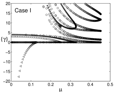
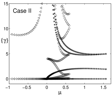
Figure 3: Illustration of the stability of the exact solutions. Shown is the eigenvalue spectrum $\{\gamma\}$ for the matrix product $A$$B$, $\nu=1$. Case I (left panel) and $N_{p}=3$ (triangles), $N_{p}=4$ (squares), $N_{p}=5$ (stars), and $N_{p}=10$ (circles). Case II (right panel) $N_{p}=3$ (triangles), $N_{p}=5$ (stars), and $N_{p}=10$ (circles).

The eigenvalue spectrum $\{\gamma\}$ of the matrices $A$$B$ and $B$$A$ determines the stability of the exact solutions. If it contains negative eigenvalues the solution is unstable. The eigenvalue spectrum always contains two eigenvalues which are zero. These eigenvalues correspond to the translational invariance ($c$) and to the invariance of the solution $\psi_{n}^{j}$ to a constant phase factor $e^{-i\delta}$ (i.e. translation in time), respectively. In Fig. 3 we show the eigenvalue spectrum $\{\gamma\}$ for the cases I and II for several periodicities $N_{p}$. It is important to note that in this figure we have $N=N_{p}$. It turns out that the spectrum $\{\gamma\}$ is independent of $c$. The figure demonstrates that for $N=N_{p}$, only the $\psi_{n}^{I}$ solution becomes unstable and this occurs only for $N_{p}=3$. For all other values of $N_{p}$ both solutions are linearly stable. This also indicates that the localized solution $\psi_{n}^{III}$ is linearly stable; and we have checked that this indeed is the case in the entire existence interval.

The solutions $\psi_{n}^{I}$, and $\psi_{n}^{II}$ exist for all lattices $N=JN_{p}$ where $J$ is a positive integer. However, we find $\psi_{n}^{I}$ to be stable only for $J=1$, while $\psi_{n}^{II}$ is stable for all $J$.

Finally, it is worth pointing out that Eq. (1) also has an exact constant amplitude solution

$$\psi_{n}(t)=\psi_{0}\exp[-i(\omega t-qn+\delta)]\,,$$ (24)

where $\delta$ is a constant and $\omega$ satisfies the nonlinear dispersion relation

$$\omega=4\sin^{2}(q/2)-\frac{\nu\mid\psi_{0}\mid^{2}}{1+\mu\mid\psi_{0}\mid^{2}}\,,$$ (25)

where the wavenumber $q=2\pi p/N_{p}$ in order to comply with the periodic boundary condition, and $p$ is an intger.

In conclusion, we have presented two spatially periodic and one spatially localized exact solutions of the DNLS equation with a saturable nonlinearity. We found these solutions to be linearly stable in most cases. We also calculated the Peierls-Nabarro barrier for the localized solution. These results are relevant for wave propagation in optical waveguides and doped fibers OP ; fibers , Bose-Einstein condensates ST as well as for many other nonlinear physical applications. Note that a related continuum version of Eq. (1), which arises in the context of the Fokker-Planck equation for a single mode laser, has been considered in Ref. SH . It would be important to search for ways of modifying the nonlinearity so that the PN barrier becomes zero–a possible route to an integrable model.

This work was supported in part by the U.S. Department of Energy.

Appendix A

In this appendix we give explicit expressions for $H$ and $P$ for the two spatially periodic solutions. While the importance of the energy expression is obvious, we would like to emphasize that the expressions for $P$ could be used as a numerical diagnostic, for instance in keeping track of a conserved quantity in a simulation involving these solutions.

Inserting the solution given by Eq. (5) into Eq. (2) we get for the energy

$${\cal H}^{I}=\frac{2}{\mu}\frac{\mbox{sn}^{2}(\beta,m)}{\mbox{cn}^{2}(\beta,m)}\bigg{(}-N_{p}\big{(}\mbox{dn}(\beta,m)-\mbox{cs}(\beta,m)Z(\beta,m)\big{)}+\left(1-\frac{\nu}{2\mu}\right)\sum_{n=1}^{N_{p}}\mbox{dn}^{2}([n+c]\beta,m)\bigg{)}$$

$$+\frac{\nu}{\mu^{2}}\sum_{n=1}^{N_{p}}\mbox{ln}\left(1+\frac{\mbox{sn}^{2}(\beta,m)}{\mbox{cn}^{2}(\beta,m)}\mbox{dn}^{2}([n+c]\beta,m)\right),$$ (26)

where $Z(\beta,m)$ is the Jacobi zeta function and cs$(\beta,m)$ = cn$(\beta,m)$/sn$(\beta,m)$. Also, use has been made of the identity Khare dn$(y,m)$dn$(y+a,m)$=dn$(a,m)-$cs$(a,m)$Z$(a,m)$+cs$(a,m)$[Z$(y+a,m)$-Z$(y,m)]$ and the fact that $\sum_{n=1}^{N_{p}}[Z(\beta(n+1+c),m)-Z(\beta(n+c),m)]=0$. From Eq. (3) we get for the power

$${\cal P}^{I}=\frac{1}{\mu}\frac{\mbox{sn}^{2}(\beta,m)}{\mbox{cn}^{2}(\beta,m)}\sum_{n=1}^{N_{p}}\mbox{dn}^{2}([n+c]\beta,m).$$ (27)

Similarly, inserting the solution given by Eq. (8) into Eq. (2) we get for the energy

$${\cal H}^{II}=\frac{2}{\mu}\frac{\mbox{sn}^{2}(\beta,m)}{\mbox{dn}^{2}(\beta,m)}\bigg{(}-N_{p}\big{(}m\,\mbox{cn}(\beta,m)-\mbox{ds}(\beta,m)Z(\beta,m)\big{)}+\left(1-\frac{\nu}{2\mu}\right)\sum_{n=1}^{N_{p}}\mbox{cn}^{2}([n+c]\beta,m)\bigg{)}$$

$$+\frac{\nu}{\mu^{2}}\sum_{n=1}^{N_{p}}\mbox{ln}\left(1+\frac{\mbox{sn}^{2}(\beta,m)}{\mbox{dn}^{2}(\beta,m)}\mbox{cn}^{2}([n+c]\beta,m)\right)$$

$$=\frac{2}{\mu}\frac{\mbox{sn}^{2}(\beta,m)}{\mbox{dn}^{2}(\beta,m)}\bigg{(}-N_{p}\big{[}m\,\mbox{cn}(\beta,m)-\mbox{ds}(\beta,m)Z(\beta,m)\big{]}+\left(1-\frac{\nu}{2\mu}\right)\big{[}-(1-m)N_{p}+\sum_{n=1}^{N_{p}}\mbox{dn}^{2}([n+c]\beta,m)\big{]}\bigg{)}$$

$$+\frac{\nu}{\mu^{2}}\bigg{(}N_{p}\mbox{ln}\left(\frac{\mbox{cn}^{2}(\beta,m)}{\mbox{dn}^{2}(\beta,m)}\right)+\sum_{n=1}^{N_{p}}\mbox{ln}\left[1+\frac{\mbox{sn}^{2}(\beta,m)}{\mbox{cn}^{2}(\beta,m)}\mbox{dn}^{2}([n+c]\beta,m)\right]\bigg{)},$$ (28)

where again $Z(\beta,m)$ is the Jacobi zeta function and ds$(\beta,m)$ = dn$(\beta,m)$/sn$(\beta,m)$. Also, use has been made of the identity Khare $m\,$cn$(y,m)$cn$(y+a,m)$=$m\,$cn$(a,m)-$ds$(a,m)$Z$(a,m)$+ds$(a,m)$ [Z$(y+a,m)$-Z$(y,m)$]. From Eq. (3) we get for the power

$${\cal P}^{II}=\frac{1}{\mu}\frac{\mbox{sn}^{2}(\beta,m)}{\mbox{dn}^{2}(\beta,m)}\sum_{n=1}^{N_{p}}\mbox{cn}^{2}([n+c]\beta,m)=\frac{1}{\mu}\frac{\mbox{sn}^{2}(\beta,m)}{\mbox{dn}^{2}(\beta,m)}\left(-N_{p}(1-m)+\sum_{n=1}^{N_{p}}\mbox{dn}^{2}([n+c]\beta,m)\right).$$ (29)

In order to get the sums over the same expressions for ${\cal H}^{II}$ and ${\cal P}^{II}$ as for ${\cal H}^{I}$ and ${\cal P}^{I}$ we have used the basic relations $\mbox{cn}^{2}(x,m)+\mbox{sn}^{2}(x,m)=1$ and $\mbox{dn}^{2}(x,m)+m\mbox{sn}^{2}(x,m)=1$. In the continuum limit (small $\beta$, large $N_{p}$) the sums may be replaced by integrals. First

$$\sum_{n=1}^{N_{p}}\mbox{dn}^{2}([n+c]\beta,m)\simeq\frac{QE(m)}{\beta}=\frac{QK(m)}{\beta}\frac{E(m)}{K(m)}=N_{p}\frac{E(m)}{K(m)},$$ (30)

where $Q=2$ in Case I and $Q=4$ in Case II. The other sum

$$\sum_{n=1}^{N_{p}}\mbox{ln}\left(1+\frac{\mbox{sn}^{2}(\beta,m)}{\mbox{cn}^{2}(\beta,m)}\mbox{dn}^{2}([n+c]\beta,m)\right)\simeq N_{p}\mbox{ln}\bigg{(}\frac{\pi\Theta^{2}(\beta,m)}{2\sqrt{1-m}K(m)\mbox{cn}^{2}(\beta,m)}\bigg{)},$$ (31)

where $\Theta(\beta,m)$ is the Jacobi theta function. For $m\rightarrow 1$, Eqs. (A1) and (A3) can be used to determine the asymptotic interaction between two nonlinear solutions given by Eq. (11).

References

(1) P.G. Kevrekidis, K.Ø. Rasmussen, and A.R. Bishop,
Int. J. Mod. Phys. B 15, 2833, (2001).
(2) H.S. Eisenberg, Y. Silberberg, R. Morandotti, A.R. Boyd, and J.S. Aitchison,
Phys. Rev. Lett. 81, 3383 (1998).
(3) A. Trombettoni and A. Smerzi, Phys. Rev. Lett. 86, 2353 (2001).
(4) S. Gatz and J. Herrmann, J. Opt. Soc. Am. B 8, 2296 (1991);
S. Gatz and J. Herrmann, Opt. Lett. 17, 484 (1992).
(5) A. Khare and U. Sukhatme, J. Math. Phys. 43, 3798 (2002);
A. Khare, A. Lakshminarayan, and U. Sukhatme, J. Math. Phys. 44, 1822 (2003);
math-ph/0306028; Pramana (Journal of Physics) 62, 1201 (2004).
(6)Handbook of Mathematical Functions with Formulas, Graphs,
and Mathematical Tables, edited by M. Abramowitz and I. A. Stegun (U.S. GPO, Washington, D.C., 1964).
(7)Solitons: An Introduction, P.G. Drazin and R.S. Johnson (Cambridge University
Press, Cambridge, 1989).
(8)Nonlinear Science: Emergence & Dynamics of Coherent
Structures, Alwyn Scott (Oxford University Press, Oxford, 1999).
(9) A. Saxena and A.R. Bishop, Phys. Rev. A 44, R2251 (1991);
J. P. Boyd, SIAM J. Appl. Math. 44, 952 (1984).
(10) O. M. Braun and Yu. S. Kivshar, Phys. Rev. B 43, 1060
(1991); Yu. S. Kivshar and D. K. Campbell, Phys. Rev. E 48, 3077
(1993).
(11) T. Dauxois and M. Peyrard, Phys. Rev. Lett. 70,
3935 (1993).
(12) A. Saxena and S. Habib, Physica D 107, 338 (1997).