Combination of anticipated and isochronous synchronization in coupled semiconductor lasers system

Abstract

Combination of two basic types of synchronization, anticipated and isochronous synchronization, is investigated numerically in coupled semiconductor lasers. Due to the combination, a synchronization of good quality can be obtained. We study the dependence of the lag time between two lasers and the synchronization quality on the converse coupling retardation time $\tau_{c21}$. When $\tau_{c21}$ is close to the difference of external cavity round trip time $\tau$ and coupling retardation time $\tau_{c12}$, the combination of anticipated and isochronous synchronization may produce a better synchronization, with a lag time proportional to $\tau_{c21}$. When $\tau_{c21}$ is largely different from $\tau-\tau_{c12}$, the combination is noneffective and even negative in some cases, with a lag time independent of $\tau_{c21}$.

I Introduction

In last few decades, much attention has been paid to chaotic synchronization because of its potential applications in wide variety of fields, especially in communications Pecora and Carroll (1990); Winful and Rahman (1990); Roy and Thornburg (1994); Sugawara et al. (1994); VanWiggeren and Roy (1998); Goedgebuer et al. (1998). Recent focus is put upon coupled semiconductor lasers operating in Low-Frequency-Fluctuation (LFF) regime Sivaprakasam and Shore (1999); Fischer et al. (2000); Fujino and Ohtsubo (2000); Ahlers et al. (1998); Mirasso et al. (1996); Annovazzi-Lodi et al. (1996), where the intensity output of the laser exhibits irregular dropout events (sisyphus effect, see Heil et al. (1998)). Sudden reduction in output (a dropout) is followed by a gradual recovery and then another dropout comes Risch and Voumard (1977); Heil et al. (1998); Henry and Kazarinov (1986); Sano (1994); Fischer et al. (1996). The interval between dropouts is irregular Hohl et al. (1995); Sukow et al. (1997); Marino et al. (2002); Buldú et al. (2004)and two lasers without interaction to each other should exhibit severally irregular and uncorrelated dropouts. When there is a coupling between two lasers by injecting part output of one laser (laser1) into the other (laser2), the two lasers may produce correlated outputs, particularly in dropout events Wallace et al. (2000). In other words Dropouts of laser1 is imaged into the output of laser2, thus dropout events of two lasers appear in the same pace, and synchronization between two lasers is achieved in this way. Such synchronization doesn’t mean always exact equality of two lasers’ outputs, but can be considered as a chaos control of laser2’s LFF behavior by laser1, in spite that complete synchronization can be obtained in special situations Voss (2000); Masoller (2001); Liu et al. (2001); Tang and Liu (2003).

Through a simple analysis of the rate equations for the unidirectional coupling lasers system, two types of synchronization has been identified Locquet et al. (2001); Locquet et al. (2002a, b); Shahverdiev and Shore (2002); Murakami and Ohtsubo (2002); Koryukin and Mandel (2002):

$$Anticipated\ Synchronization(AS):\quad I_{2}(t-\tau)=I_{1}(t-\tau_{c12})$$ (1)

$$Isochronous\ Synchronization(IS):\quad I_{2}(t)=I_{1}(t-\tau_{c12})$$ (2)

System may choose one type of synchronization to exhibit, and the other synchronization behavior is hidden. Which type is chosen is determined by the competition between two types. The winner is shown and the loser is hidden. Transition from one type to the other may occur when operating parameters are changed Locquet et al. (2002b); Wu and Zhu (2003); Sivaprakasam et al. (2002). But virtually there is not only competition but also cooperation or combination between two types of synchronization, especially when the problem is extended to the field of complex network with delayed feedback and coupling Barahona and Pecora (2002); Atay and Jost (2004); Albert and Barabási (2002). In this paper, after some brief introduction to the two basic types of synchronization, the synchronization combination phenomenon is discussed. To our best knowledge, this is the first paper to discuss the combination of the two basic types of chaotic synchronization in coupled semiconductor lasers system.

II Anticipated and Isochronous Synchronization

The two basic types of synchronization are reviewed in this section.

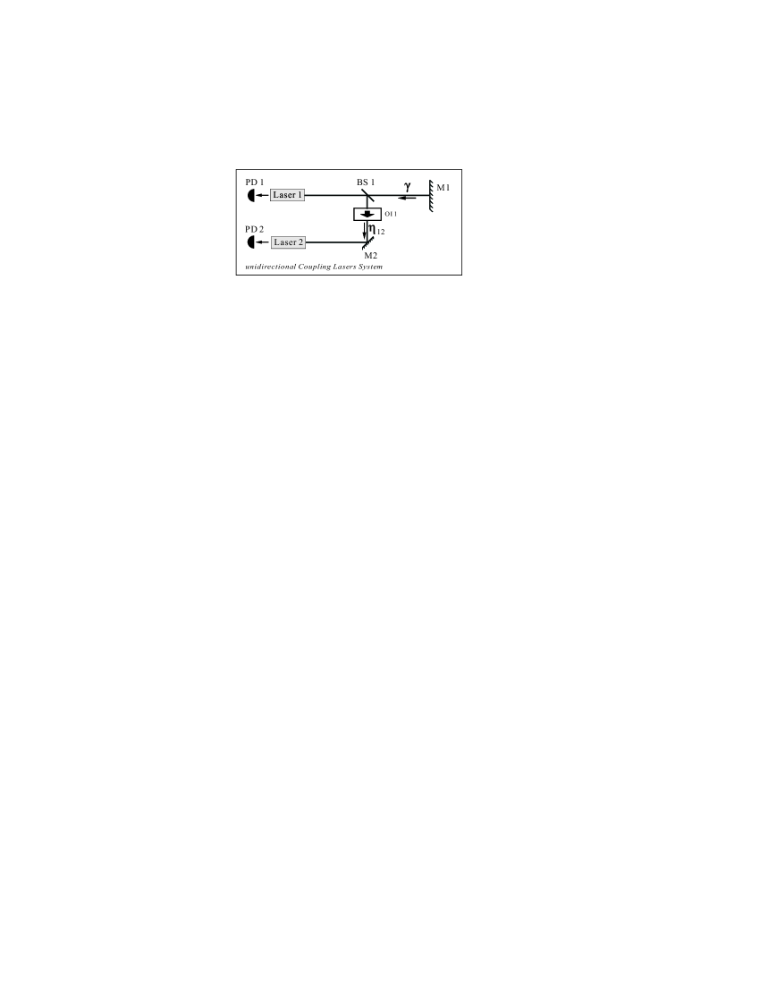
Figure 1: Schematic representation of unidirectional coupling lasers system, where two basic types of synchronization are shown typically.

The unidirectional coupling lasers system is shown in Fig.1. Part output of laser1 is injected back as a feedback by a mirror M1. Another part is injected into laser2 via a beam splitter BS1, an optical isolator OI1 (ensure there is no light from laser2 to enter laser1 and alter the dynamics of laser1) and another mirror M2. No feedback is used in laser2. Photo diodes (PD1, 2) is used to detect outputs of two lasers respectively. Feedback rate is labelled by $\gamma$, $\eta_{12}$ is coupling strength from laser1 to laser2.

Numerical simulation is performed by LK equations for the complex electric fields $E$ and normalized carrier densities $N$ Lang and Kobayashi (1980).

$$\frac{dE_{1}}{dt} = k(1+i\alpha)[G_{1}-1]E_{1}(t)+\gamma_{1}E_{1}(t-\tau)e^{(-i\omega_{1}\tau)}+\beta\xi_{1}(t)$$ (3)

$$\frac{dN_{1}}{dt} = \frac{j-N_{1}-G_{1}|E_{1}|^{2}}{\tau_{n}}$$ (4)

$$\frac{dE_{2}}{dt} = k(1+i\alpha)[G_{2}-1]E_{2}(t)+\eta_{12}E_{1}(t-\tau_{c12})e^{[-i(\omega_{1}\tau_{c12}+\triangle\omega t)]}+\beta\xi_{2}(t)$$ (5)

$$\frac{dN_{2}}{dt} = \frac{j-N_{2}-G_{2}|E_{2}|^{2}}{\tau_{n}}$$ (6)

Where subscripts 1 and 2 denote Laser1 and Laser2 respectively. The second term in Eq. (1) corresponds to the feedback in Laser1, and the second term in Eq. (3) corresponds to the coupling from laser1 to laser2. $k$ is the cavity loss, $\alpha$ the linewidth enhancement factor, $G=N/(1+\epsilon|E|^{2})$ is the optical gain, $\epsilon$ is the gain saturation coefficient, $\omega$ is the optical frequency without feedback, $\triangle\omega=\omega_{2}-\omega_{1}$ is the frequency detuning, $\xi$ is independent complex Gaussian white noise, and $\beta$ measures the noise strength, $j$ is the normalized injection current, and $\tau_{n}$ is the carrier lifetime. For simplicity, we may choose $\beta_{1}=\beta_{2}=0$. Two types of synchronization are shown in following two cases respectively.

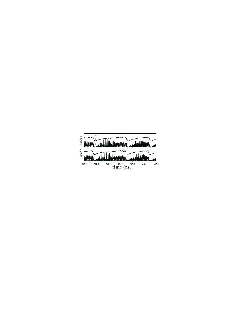
Figure 2: Time traces of two unidirectional coupling lasers operating in the LFF regime, typically showing anticipated synchronization with parameters: $\eta_{12}=\gamma=8ns^{-1}$, $\tau=7ns$, $\tau_{c12}=4ns$, $j=1.003$, $\alpha=5$, $k=500ns^{-1}$, $\tau_{n}=1ns$. Vertically shifted low-pass-filtered ones are plotted in solid lines to emulate the experimental detection and exhibit the dropout events clearly Fischer et al. (1996).

In the first case, a typical AS (anticipated synchronization) is shown with parameters: $\eta_{12}=\gamma=8ns^{-1}$, $\tau=7ns$ ($\tau$ is external cavity round trip time in laser1), $\tau_{c12}=4ns$ ($\tau_{c12}$ is the time for light to travel from laser1 to laser2). The intensity outputs of two lasers are plotted in Fig. 2. The two lasers are both operating in LFF regime, where sudden output reduction (a dropout) appears, followed by a gradual recovery, and then another dropout comes. Intervals between dropouts is irregular. To remove the fluctuations in high frequencies so as to make the dropout events clearer, the low-pass-flitter diagrams are also plotted and shifted upward. The dropout events is labelled by short dotted lines.

As clearly shown in Fig. 2, the two lasers undergo dropouts in the same pace due to the coupling and synchronization is achieved. In addition, 3ns before every dropout in laser1, there is always a corresponding dropout in laser2, as if laser2 can predict the future state of laser1 in spite that laser2’s chaotic dynamics is driven by laser1. This is a typical AS, satisfying Eq. (1).

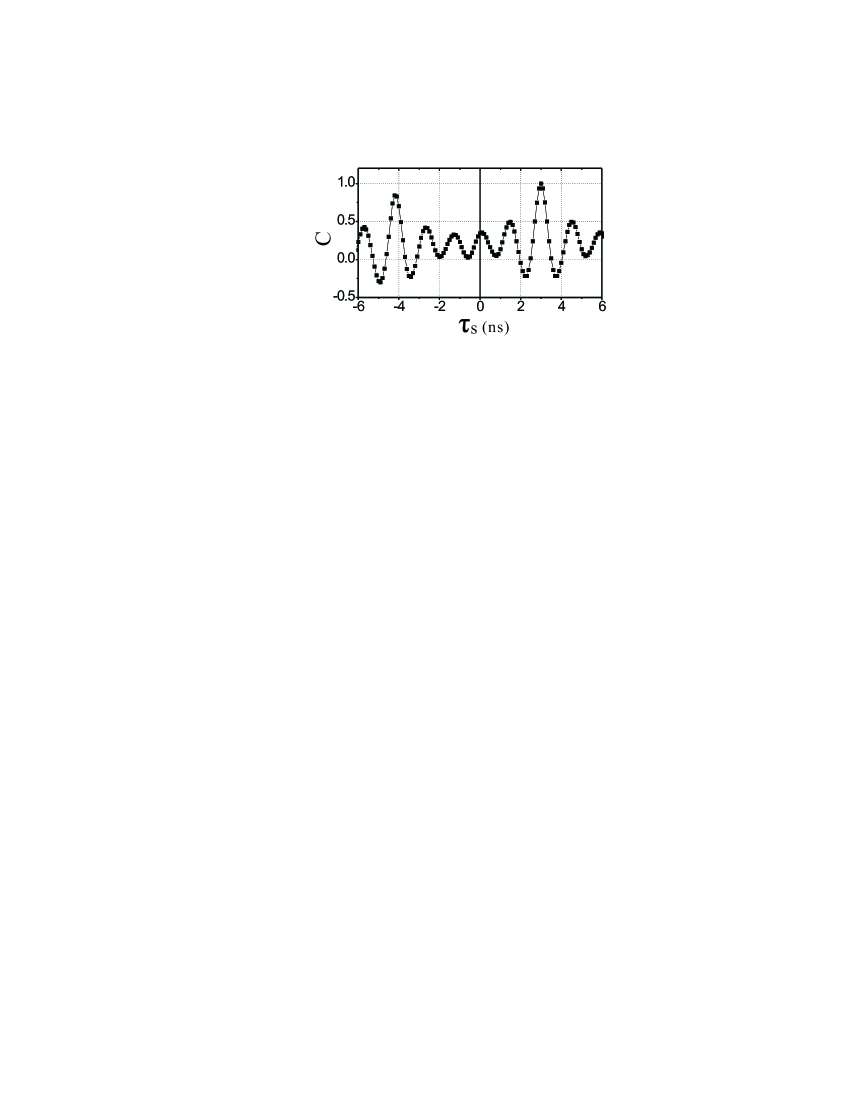
Figure 3: plot of correlation function C as a function of shift time $\tau_{s}$, corresponding to the typical anticipated synchronization in Fig. 2.

In Fig. 3 correlation function C between two lasers’ outputs as a function of shift time ($\tau_{s}$) is also plotted. C is defined as follows:

$$C(\tau_{s})=\frac{\langle[I_{1}(t+\tau_{s})-\langle I_{1}\rangle][I_{2}(t)-\langle I_{2}\rangle]\rangle}{\{\langle[I_{1}(t)-\langle I_{1}\rangle]^{2}\rangle\langle[I_{2}(t)-\langle I_{2}\rangle]^{2}\rangle\}^{1/2}}$$ (7)

At $\tau_{s}=3ns$ there is a peak. This peak indicates that a strong correlation can be obtained when laser2 is shifted backward by 3ns. Obviously this peak corresponds to the AS in Fig. 2.

Besides the right peak, there is another peak at $\tau_{s}\approx-4ns$. (It is noted that $\tau_{c12}=4ns$ in our simulation. This peak indicates that shifting laser2 forward by $\tau_{c12}$ also can produce a strong correlation. This left peak satisfies Eq. (1) and corresponds to IS. Although only AS is shown in Fig. 2, two-peaks configuration in correlation plot implies the existence of IS. Only because the right peak is higher (indicating that the anticipated synchronization quality is better), AS is the winner in the competition with IS, and IS behavior is hidden.

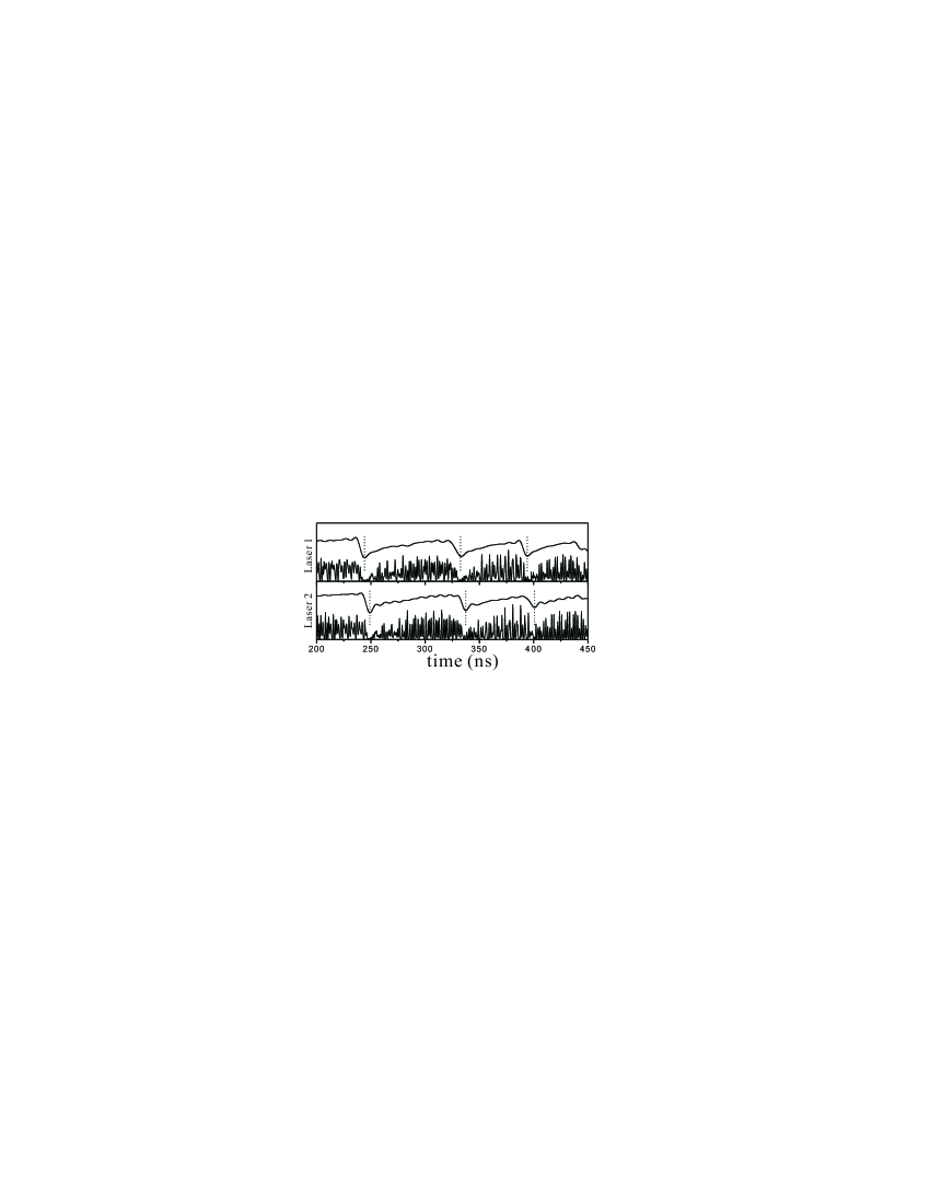
Figure 4: Time traces of two unidirectional coupling lasers typically showing isochronous synchronization with parameters: $\eta_{12}=5ns^{-1}$, other parameters are the same as in Fig. 2.

In the second case, a typical IS (isochronous synchronization) is shown with parameters: $\eta_{12}=8ns^{-1}$, $\gamma=5ns^{-1}$, $\tau=7ns$, $\tau_{c12}=4ns$, namely only $\gamma$ is decreased a little. Outputs of two lasers and vertically-shifted low-pass-filtered diagrams are plotted in Fig. 4, ranging from 200ns to 450ns. Every dropout in laser1 leads the corresponding dropout by about 4ns (We note $\tau_{c12}=4ns$). So there is a typical IS between the two lasers, satisfying Eq. (2). This synchronization is induced by the fact that the unidirectional coupling is sufficient for the laser1 to drive the dynamics of the laser2 and lead to a locking-state phenomenon.

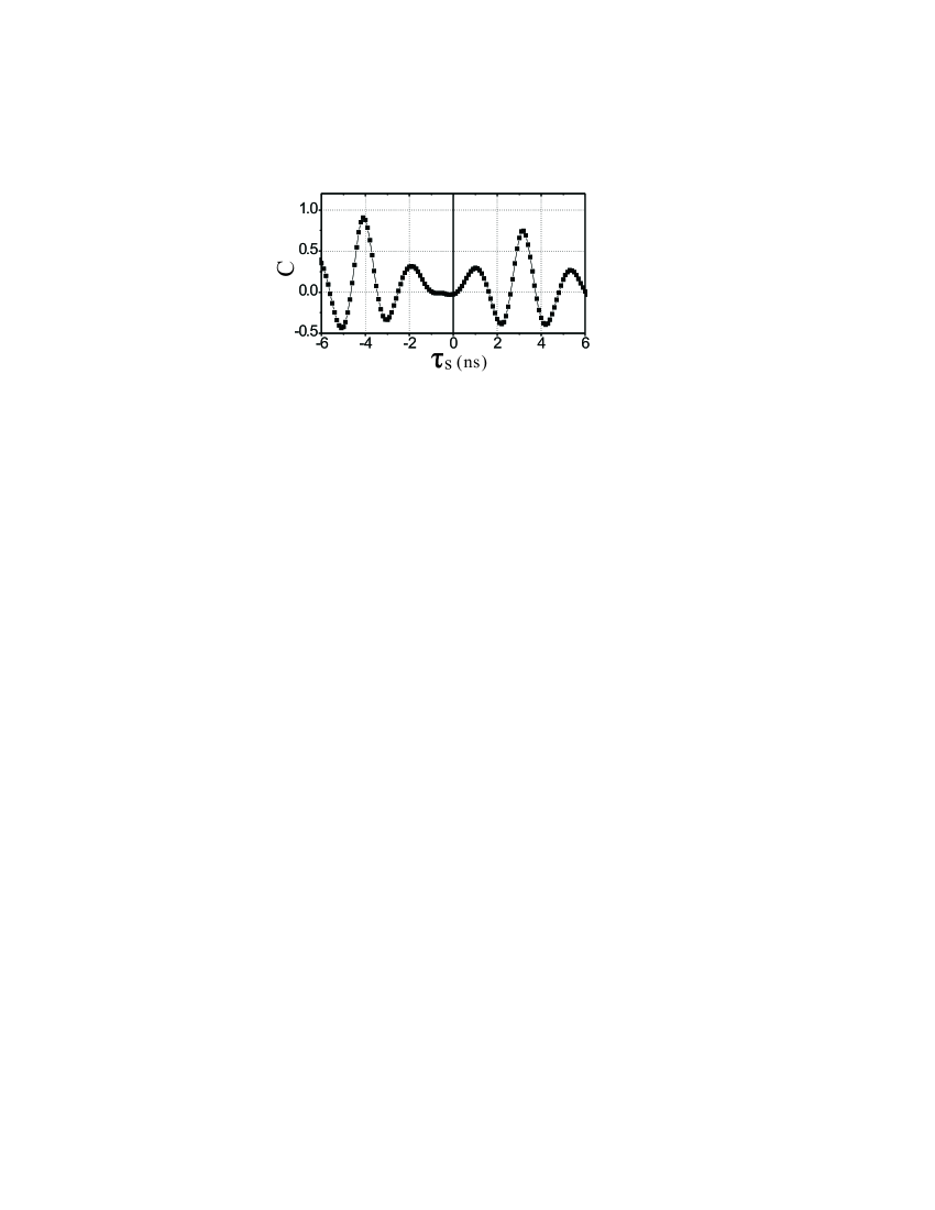
Figure 5: plot of correlation function C as a function of shift time $\tau_{s}$, corresponding to the typical isochronous synchronization in Fig. 4.

Fig. 5 is the correlation plot. It is very easy to identify the two peaks. The left peak corresponds to IS and the right one corresponds to AS. Only because the left peak is higher than the right one (indicating that the isochronous synchronization quality is better), AS is the loser in the competition with IS and has been hidden. Hence it is clearly seen in Fig. 4 that only IS is shown.

According to above discussion, which type of synchronization is shown, AS or IS, is determined by their competition. The winner’s behavior is shown, while the loser still exists in the system but has been hidden.

III Synchronization Combination

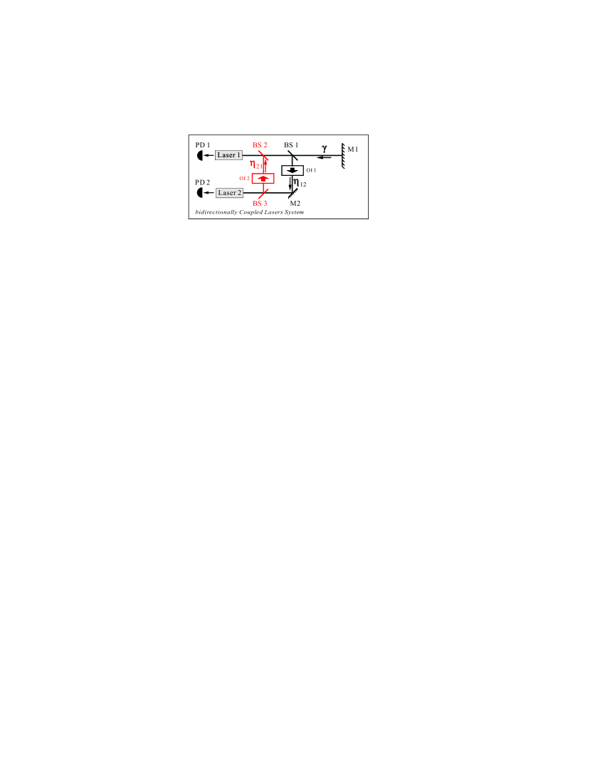
Figure 6: Schematic representation of bidirectional coupling lasers system, where the combination of anticipated and isochronous synchronization is investigated. The coupling from laser1 to laser2 travels via BS1, OI1 and M2, while the converse coupling from laser2 to laser1 travels via BS3, OI2 and BS2.

AS and IS not only compete but also cooperate with each other, i.e. their combination. In this section such combination is discussed. the model under our following discussion is almost the same as the second case in the previous section except that a converse coupling with coupling strength $\eta_{21}$ is used as shown in Fig. 6 with parameters: $\eta_{21}=\eta_{12}=8ns^{-1}$, $\gamma=5ns^{-1}$. Two optical isolators are used to make sure that both couplings are unidirectional, then $\tau_{c21}\neq\tau_{c12}$, which is helpful in following analysis. $\tau_{c21}$ is the time taken for the light to travel from laser2 back to laser1.

Then the right correlation peak appears because of a combination of two factors:

(1)Before adding the converse coupling, there has been an AS: $I_{2}(t-\tau)=I_{1}(t-\tau_{c12})$, where laser2 lags laser1 by the time $\tau_{s}=\tau-\tau_{c12}$.

(2)After adding the converse coupling, there is also an IS due to the converse coupling from laser2 to laser1: $I_{1}(t)=I_{2}(t-\tau_{c21})$, where laser2 lags laser1 by the time $\tau_{s}=\tau_{c21}$.

We may choose: $\tau=7ns$, $\tau_{c12}=4ns$, and $\tau_{c21}=3ns$, then $\tau_{c21}=\tau-\tau_{c12}$, and there will be a combination of AS with IS at $\tau_{s}=3ns$.

The dynamical behavior of bidirectional coupling laser1 (with a external feedback)and laser2 (solitary) is described by Eq. (8, 9) and Eq. (5, 6) respectively.

$$\frac{dE_{1}}{dt} = k(1+i\alpha)[G_{1}-1]E_{1}(t)+\gamma_{1}E_{1}(t-\tau)e^{(-i\omega_{1}\tau)}+\eta_{21}E_{2}(t-\tau_{c21})e^{[-i(\omega_{2}\tau_{c21}-\triangle\omega t)]}+\beta\xi_{1}(t)$$ (8)

$$\frac{dN_{1}}{dt} = \frac{j-N_{1}-G_{1}|E_{1}|^{2}}{\tau_{n}}$$ (9)

where the third term in Eq. (8) is added for the converse coupling.

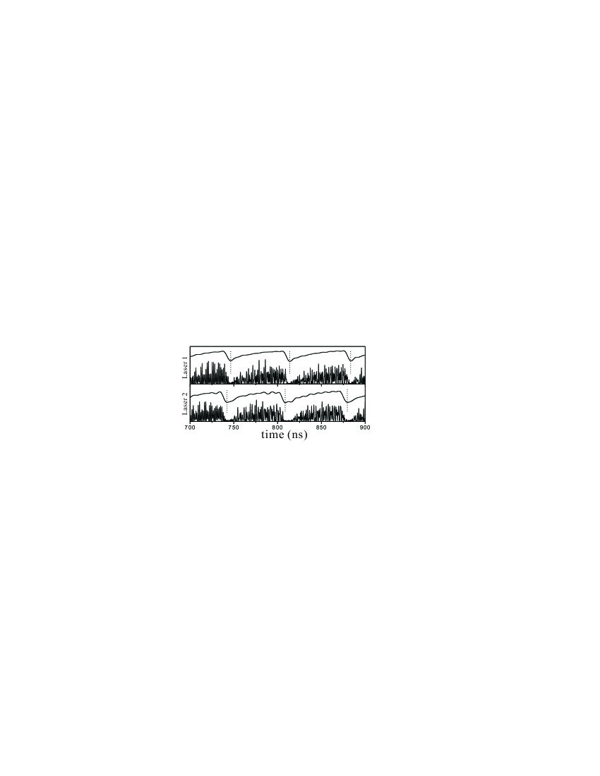
Figure 7: Time traces of two lasers, showing the effect of the combination of anticipated and isochronous synchronization, laser2 is seen to synchronize and lead laser1. parameters are: $\eta_{21}=8ns^{-1}$, $\tau_{c21}=3ns$, and other parameters are the same as in Fig. 4.

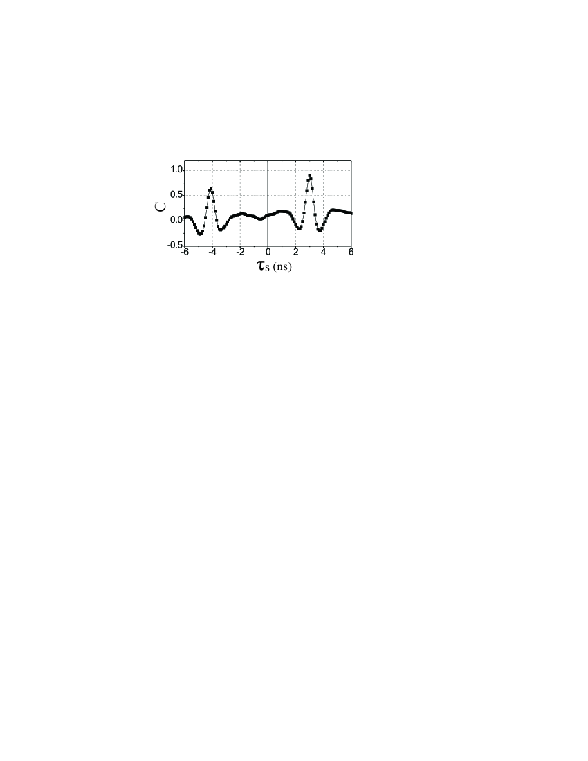
Figure 8: plot of correlation function C as a function of shift time $\tau_{s}$, corresponding to the combination of anticipated and isochronous synchronization in Fig. 7.

Numerical simulation is shown in Figs. 7 and 8. As expected, in Fig. (7) 3ns before every dropouts of laser1 there has been a dropout in laser2 inevitably. Synchronization between two lasers is achieved and Laser2 leads laser1 by 3ns.

That Laser2 can predict the future dynamical behavior of laser1 results from the combination of two basic types of synchronization behavior, AS and IS. The effect of combination is also exhibited by the correlation plot Fig. 8. The right correlation peak at $\tau_{s}=3ns$, reflecting the effect of combination of AS and IS, is higher. While the left peak at $\tau_{s}\approx-4ns$ reflecting IS produced by only the coupling from laser1 to laser2 is lower and its corresponding dynamical behavior is hidden. So only the combination synchronization is shown.

It seems that the matching condition $\tau_{c21}=\tau-\tau_{c12}$ makes the combination of AS and IS create a strong correlation and consequent combination synchronization. For further discussion about the effect of combination of AS and IS, a more general situation where $\tau_{c21}\neq\tau-\tau_{c12}$ is concerned by moving the branch of the converse coupling so that $\tau_{c21}$ is modified.

In the following discussion, combination synchronization quality $Q_{c}$ and its characteristic time scale $T_{c}$ are investigated:

$$Q_{c}=\max(C(\tau_{s})),\quad\tau_{s}>0$$ (10)

$$C(T_{c}))=Q_{c}$$ (11)

where $T_{c}$ is the lag time between two lasers.

(1) In AS, laser1 lags laser2 by the time dependent on the difference of the external cavity round trip time of laser1 and the coupling retardation time , i.e. $\tau-\tau_{c12}$, independent on the converse coupling retardation time $\tau_{c21}$. When $\tau_{c21}$ is increased, the lag time should almost remain unchanged.

(2) In IS, laser1 lags laser2 by the time dependent on the converse coupling retardation time $\tau_{c21}$. When $\tau_{c21}$ is increased, the lag time should be increased proportionally.

In combination of AS and IS, whether the lag between two lasers ($T_{c}$) is changed proportionally or unchanged when $\tau_{c21}$ is increased?

Figure 9: shows the dependence of $T_{c}$ and $Q_{c}$ on the converse coupling retardation time $\tau_{c21}$ ranged from 2.4ns to 3.6ns. Five regions are identified. All the parameters are the same as in Fig. 7 except for the variable $\tau_{c21}$.

Fig. 9 shows the dependence of $T_{c}$ (a) and combination synchronization quality $Q_{c}$ (b) on the converse coupling retardation time $\tau_{c21}$. The interesting results show the range of $\tau_{c21}$ from 2.4ns to 3.6ns can be divided into five regions, labelled by I-V. In region I and V, $T_{c}$ is unchanged and always stay near 3.0ns, that indicates when $\tau-\tau_{c12}$ and $\tau_{c21}$ is largely different as in region I and V, AS behavior is exhibited and more prominent in the combination of AS and IS. Furthermore, it is seen in Fig. 9(b) that corresponding $Q_{c}$ is near the quality of only AS (The quality of only AS is shown by the height of the right peak in Fig. 5, where the converse coupling is still not added, and is also lined out in Fig. 9(b) by a straight line.) It seems that when two characteristic time scales $\tau-\tau_{c12}$ and $\tau_{c21}$ are largely different, The combination effect is not so great to enhance the synchronization quality. In region III where $\tau_{c21}$ is close to $\tau-\tau_{c12}$, $T_{c}$ always approximately equals to $\tau_{c21}$ ($T_{c}\approx\tau_{c21}$), presenting a striking contrast with Region I and V. The fact that $T_{c}$ increases with $\tau_{c21}$ in region III implies IS behavior is prominent and the decisive force in the combination of AS and IS. In addition, the quality of the combination synchronization goes over the straight line mostly, indicating the combination of IS and AS has produced a better synchronization than only AS in most of region III. The maximum efficiency of the combination is obtained at about $\tau_{c21}=3ns$ ($\tau-\tau_{c12}=3ns$). Regions II and IV are transition regions. $T_{c}$ falls rapidly from $\tau-\tau_{c12}$ to $\tau_{c21}$ in region II, and from $\tau_{c21}$ back to $\tau-\tau_{c12}$ in region IV. In this transition regions the situation that neither AS nor IS is prominent in the combination may occur, where the quality of the resulting combination synchronization is even worse than only AS, especially in region II.

IV Discussion

We note that In Fig. 7 where the combination synchronization is demonstrated, the both couplings are of the same strength, i.e. $\eta_{12}=\eta_{21}$. If the feedback in laser1 is removed, the system will turn to be a typical Face-to-Face (F2F) model Heil et al. (2001); Mulet et al. (2002). In F2F model, synchronization can be obtained with a time lag between two lasers. And the leader role switches from one laser to the other randomly and continuously because of the symmetry. Without the explanation from the viewpoint of synchronization combination, it is very hard to understand why laser2 will always leads laser1 after a delayed feedback is added in laser1.

A simple analysis of the rate equations for the unidirectional lasers system has identified the required matching condition $\eta_{12}=\gamma$ (no feedback in laser2) necessary for the existence of AS. We note this condition is necessary for the complete synchronization. In fact, when the stringent matching condition is not satisfied AS still exists, but it is not so good and always hidden behind. As shown in Fig. 7, such not so good AS has even become an important factor in the synchronization combination.

Sivaprakasam et al experimentally demonstrated a very interesting synchronization phenomenon between two bidirectional coupling lasers Sivaprakasam et al. (2001); Rees et al. (2003). Their setup configuration is the same as Fig. 6 of this paper except for $\tau_{c12}=\tau_{c21}$ in their setup. They found experimentally that ”slave” can predict the future state of the ”master” and the corresponding ”anticipating time” always equals to the coupling retardation time. We thind the experimentally obtained synchronization may arise from the combination of synchronization. And in region III of Fig. 9 of this paper, $T_{c}=\tau_{c21}$ is in good agreement with their experimental result.

References

- Pecora and Carroll (1990) L. M. Pecora and T. L. Carroll, Phys. Rev. Lett. 64, 821 (1990).
- Winful and Rahman (1990) H. G. Winful and L. Rahman, Phys. Rev. Lett. 65, 575 (1990).
- Roy and Thornburg (1994) R. Roy and K. S. Thornburg, Phys. Rev. Lett. 72, 2009 (1994).
- Sugawara et al. (1994) T. Sugawara, M. Tachikawa, T. Tsukamoto, and T. Shimizu, Phys. Rev. Lett. 72, 3502 (1994).
- VanWiggeren and Roy (1998) G. D. VanWiggeren and R. Roy, Science 279, 1198 (1998).
- Goedgebuer et al. (1998) J.-P. Goedgebuer, L. Larger, and H. Porte, Phys. Rev. Lett. 80, 2249 (1998).
- Sivaprakasam and Shore (1999) S. Sivaprakasam and K. A. Shore, Opt. Lett. 24, 466 (1999).
- Fischer et al. (2000) I. Fischer, Y. Liu, and P. Davis, Phys. Rev. A 62, 011801(R) (2000).
- Fujino and Ohtsubo (2000) H. Fujino and J. Ohtsubo, Opt. Lett. 25, 625 (2000).
- Ahlers et al. (1998) V. Ahlers, U. Parlitz, and W. Lauterborn, Phys. Rev. E 58, 7208 (1998).
- Mirasso et al. (1996) C. R. Mirasso, P. Colet, and P. Garcia-Fernández, IEEE Photon. Electron. Lett. 8, 299 (1996).
- Annovazzi-Lodi et al. (1996) V. Annovazzi-Lodi, S. Donati, and A. Scire, IEEE J. Quantum Electron. 32, 953 (1996).
- Heil et al. (1998) T. Heil, I. Fischer, and W. Elsäer, Phys. Rev. A 58, R2672 (1998).
- Risch and Voumard (1977) C. Risch and C. Voumard, J. Appl. Phys. 48, 2083 (1977).
- Henry and Kazarinov (1986) C. H. Henry and R. F. Kazarinov, IEEE J. Quantum Electron. 22, 294 (1986).
- Sano (1994) T. Sano, Phys. Rev. A 50, 2719 (1994).
- Fischer et al. (1996) I. Fischer, G. H. M. van Tartwijk, A. M. Levine, W. Elsässer, E. Göbel, and D. Lenstra, Phys. Rev. Lett. 76, 220 (1996).
- Hohl et al. (1995) A. Hohl, H. J. C. van der Linden, and R. Roy, Opt. Lett. 20, 2396 (1995).
- Sukow et al. (1997) D. W. Sukow, J. R. Gardner, and D. Gauthier, Phys. Rev. A 56, R3370 (1997).
- Marino et al. (2002) F. Marino, M. Giudici, S. Barland, and S. Balle, Phys. Rev. Lett. 88, 040601 (2002).
- Buldú et al. (2004) J. M. Buldú, J. García-Ojalvo, and M. C. Torrent, Phys. Rev. E 69, 046207 (2004).
- Wallace et al. (2000) I. Wallace, D. Yu, W. Lu, and R. G. Harrison, Phys. Rev. A 63, 013809 (2000).
- Voss (2000) H. U. Voss, Phys. Rev. E 61, 5115 (2000).
- Masoller (2001) C. Masoller, Phys. Rev. Lett. 86, 2782 (2001).
- Liu et al. (2001) Y. Liu, Y. Takiguchi, P. Davis, T. Aida, S. Saito, and J. M. Liu, Appl. Phys. Lett. 80, 4306 (2001).
- Tang and Liu (2003) S. Tang and J. M. Liu, Phys. Rev. Lett. 90, 194101 (2003).
- Locquet et al. (2001) A. Locquet, F. Rogister, M. Sciamanna, P. Mégret, and M. Blondel, Phys. Rev. E 64, 045203 (2001).
- Locquet et al. (2002a) A. Locquet, C. Masoller, P. Mégret, and M. Blondel, Opt. Lett. 27, 31 (2002a).
- Locquet et al. (2002b) A. Locquet, C. Masoller, and C. R. Mirasso, Phys. Rev. E 65, 056205 (2002b).
- Shahverdiev and Shore (2002) E. M. Shahverdiev and K. A. Shore, Phys. Lett. A 295, 217 (2002).
- Murakami and Ohtsubo (2002) A. Murakami and J. Ohtsubo, Phys. Rev. A 65, 033826 (2002).
- Koryukin and Mandel (2002) I. V. Koryukin and P. Mandel, Phys. Rev. E 65, 026201 (2002).
- Wu and Zhu (2003) L. Wu and S. Zhu, Phys. Lett. A 315, 101 (2003).
- Sivaprakasam et al. (2002) S. Sivaprakasam, P. S. Spencer, P. Rees, and K. A. Shore, Opt. Lett. 27, 1250 (2002).
- Barahona and Pecora (2002) M. Barahona and L. M. Pecora, Phys. Rev. Lett. 89, 054101 (2002).
- Atay and Jost (2004) F. M. Atay and J. Jost, Phys. Rev. Lett. 92, 144101 (2004).
- Albert and Barabási (2002) R. Albert and A.-L. Barabási, Rev. Mod. Phys. 74, 47 (2002).
- Lang and Kobayashi (1980) R. Lang and K. Kobayashi, IEEE J. Quantum Electron. 16, 347 (1980).
- Heil et al. (2001) T. Heil, I. Fischer, W. Elsässer, J. Mulet, and C. R. Mirasso, Phys. Rev. Lett. 86, 795 (2001).
- Mulet et al. (2002) J. Mulet, C. Masoller, and C. R. Mirasso, Phys. Rev. A 65, 063815 (2002).
- Sivaprakasam et al. (2001) S. Sivaprakasam, E. M. Shahverdiev, P. S. Spencer, and K. A. Shore, Phys. Rev. Lett. 87, 154101 (2001).
- Rees et al. (2003) P. Rees, P. S. Spencer, I. Pierce, S. Sivaprakasam, and K. A. Shore, Phys. Rev. A 68, 033818 (2003).