Phase-space correlations of chaotic eigenstates

Abstract

It is shown that the Husimi representations of chaotic eigenstates are strongly correlated along classical trajectories. These correlations extend across the whole system size and, unlike the corresponding eigenfunction correlations in configuration space, they persist in the semiclassical limit. A quantitative theory is developed on the basis of Gaussian wavepacket dynamics and random-matrix arguments. The role of symmetries is discussed for the example of time-reversal invariance.

Chaotic eigenfunctions and in particular their localization and correlation statistics are a topic of continuing interest Berry (1977); Mirlin (2000); Heller (1984); Prigodin (1995); Falko and Efetov (1996); Hortikar and Srednicki (1998); Hannay (1998). Applications include classical, mesoscopic and pure quantum systems such as optical, mechanical and microwave resonators G. Hackenbroich et al. (2001); K. Schaadt et al. (2003); Kudrolli et al. (1995), electron transmission and interaction in chaotic quantum dots Alhassid (2000); J. P. Bird et al. (1999), and decay and fluctuations of heavy nuclei V. Zelevinsky et al. (1996). One foundation of eigenfunction statistics is the random-wave model of Berry Berry (1977) which is essentially equivalent to random-matrix theory (RMT) Mirlin (2000). Within RMT the eigenfunction components in an arbitrary basis are uncorrelated Gaussians. Current research is frequently aiming at deviations from RMT due to the specific dynamics. Prominent examples are scarring by periodic orbits Heller (1984) or long-range correlations Hortikar and Srednicki (1998). As classical dynamics takes place in phase space, representations of eigenstates via Husimi or Wigner functions seem appropriate, and recently some of their statistical properties have attracted a lot of attention Hannay (1998). Surprisingly this does not apply to dynamically induced correlations although numerous studies of the corresponding spatial correlations demonstrate their relevance Prigodin (1995); Hortikar and Srednicki (1998); Falko and Efetov (1996), and although there are systems where a direct relation between phase-space correlations and measurable quantities must be expected. For example, in optical resonators G. Hackenbroich et al. (2001) the power emitted at a certain point of the boundary depends strongly on the angle of incidence of the wave (total internal reflection). Also in quantum dots effects of eigenfunction directionality have been measured using tilted leads J. P. Bird et al. (1999).

In this paper we analyze for the first time dynamical correlations between points in phase space. Our results are surprising in view of the fact that spatial two-point correlators of eigenfunction amplitudes or densities vanish in the semiclassical limit $\hbar\to 0$ for any $x\neq x^{\prime}$ fn (1). In contrast we find strong and semiclassically persistent correlations between phase-space points $\xi\neq\xi^{\prime}$ ($\xi=(x,p)$) where the distance between $x$ and $x^{\prime}$ can be of the order of the system size. This is no contradiction since $\langle\psi(x)\psi(x^{\prime})\rangle=0$ does not imply that $\psi(x)$ and $\psi(x^{\prime})$ are statistically independent; it just means that there are no linear correlations in configuration space. In other words, although the existence of dynamically induced correlations cannot be a matter of the chosen basis they turn out to be most relevant in phase space.

In our approach we make use of methods which proved successful in studies of eigenfunction scarring. We will see that Gaussian wave packet dynamics Heller (1991) can also be applied to study eigenfunction properties which are not at all related to periodic orbits. As in nonlinear scarring Heller (1984) we have to supplement short-time dynamics by RMT in order to get a complete theory. However, the new context requires to do so in a technically different way.

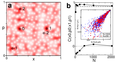
Figure 1: (a) An eigenstate of a chaotic torus map quantized with $N=256$ is shown in Husimi representation. A classical trajectory $\xi_{t}=(x_{t},p_{t})$ of the same map is marked by circles with label $t$. Inset of (b): In a scatter plot the values of the Husimi density at $\xi_{0}$ and $\xi_{1}$ cluster near the diagonal which indicates strong correlation. (b) The correlation coefficient is shown with circles as function of $N$. The dashed line is the prediction of Eq. (13). The squares show that spatial density correlations between the corresponding positions $x_{0}$ and $x_{1}$ vanish as $N\to\infty$.

We introduce our main result with a numerical example. Fig. 1a shows the Husimi representation of an eigenstate of a quantum kicked rotor,

$$\hat{U}={\rm e}^{-2\pi{\rm i}\,V(\hat{x})/h}\,{\rm e}^{-2\pi{\rm i}\,T(\hat{p})/h}\,.$$ (1)

The unitary matrix $\hat{U}$ has dimension $N\equiv h^{-1}$ and quantizes a classical map on the torus ($x+1\equiv x$, $p+1\equiv p$),

$$x_{t+1}=x_{t}+T^{\prime}(p_{t})\qquad p_{t+1}=p_{t}-V^{\prime}(x_{t+1}).$$ (2)

We choose $T(p)=p^{2}/2$ and a potential for which this map is globally chaotic fn (2). Therefore the eigenstates of $\hat{U}$ fill the entire phase space more or less uniformly. The fluctuations on this background are the object of our interest. In Fig. 1a we observe patches of high or low density which are typically of the size of a Planck cell $h$. Besides this well-known local correlation Hannay (1998), the figure suggests the existence of long-range correlations along the trajectories of the underlying classical dynamics. One such trajectory $\xi_{t}$ (not periodic!) is indicated by circles. The point $\xi_{0}$ is close to a maximum of the density, and we observe that also at the points $\xi_{t}$ the Husimi density has values above the average, at least for $-1\leq t\leq 2$. A scatter plot of the densities at $\xi_{0}$ and $\xi_{1}$ shows that this is no coincidence (inset of Fig. 1b). The corresponding correlation coefficient (circles in Fig. 1b) is as high as $0.94$ although the points $\xi_{0}$ and $\xi_{1}$ are far apart and not related by any symmetry. This is in strong contrast to the absence of long-range correlations in position or momentum representation in the semiclassical limit, which is expected from previous studies Prigodin (1995); Hortikar and Srednicki (1998); Falko and Efetov (1996) and confirmed in Fig. 1b for our model (squares).

The existence of dynamical correlations in phase space can be derived from Gaussian wave packet dynamics Heller (1991). For the special case of the quantum map Eq. (1) this standard approach is formulated as follows. The wave function of a general Gaussian state centered in phase space at $\xi_{0}=(x_{0},p_{0})$ has the form

$$g(\xi_{0},\Delta\xi,{\cal N},s;x)={\cal N}{\rm e}^{-{\cal A}_{\Delta\xi,s}{(x-x_{0})^{2}}+{\rm i}{p_{0}(x-x_{0})/\hbar}}$$ (3)

where ${\cal A}$, ${\cal N}$ are complex. The prefactor ${\cal N}$ accounts for normalization and an overall phase while

$${\cal A}_{\Delta\xi,s}=(2{\Delta_{x}})^{-2}\left({1+{s(2{\rm i}/\hbar)}\sqrt{{\Delta_{x}^{2}}{\Delta_{p}^{2}}-{\hbar^{2}\!/4}}}\right)$$ (4)

depends on the uncertainties of position and momentum, $\Delta\xi=[{\Delta_{x}},{\Delta_{p}}]$, and on a sign $s=\pm 1$. We assume that both, $\Delta_{x}$ and $\Delta_{p}$, are much smaller than any relevant classical scale fn (3). In this case and within the semiclassical approximation (stationary phase approximation for $N\to\infty$) application of the propagator (1) preserves the Gaussian form of the wave function,

$$\hat{U}\,|g(\xi_{0},\Delta\xi_{0},{\cal N}_{0},s_{0})\rangle=|g(\xi_{1},\Delta\xi_{1},{\cal N}_{1},s_{1})\rangle.$$ (5)

In this equation $\xi_{1}$ is the classical iterate of $\xi_{0}$. Position and momentum uncertainties transform as

$${\Delta_{x}^{2}}_{1} = {\Delta_{x}^{2}}_{0}-2s_{0}T_{0}^{\prime\prime}\sqrt{{\Delta_{x}^{2}}_{0}{\Delta_{p}^{2}}_{0}-\hbar^{2}\!/4}+{\Delta_{p}^{2}}_{0}{T_{0}^{\prime\prime}}^{2}$$ (6)

$${\Delta_{p}^{2}}_{1} = {\Delta_{p}^{2}}_{0}+2s_{0}^{\prime}{V_{1}^{\prime\prime}}\sqrt{{\Delta_{x}^{2}}_{1}{\Delta_{p}^{2}}_{0}-{\hbar^{2}\!/4}}+{\Delta_{x}^{2}}_{1}{V_{1}^{\prime\prime}}^{2}$$ (7)

and also for ${\cal N}_{1}$ and $s_{1}$ semiclassical expressions are found. In a chaotic system the growth of the uncertainties under repeated application of Eqs. (6), (7) will be dictated by the classical Lyapunov exponent $\lambda$ after a short initial period because then $\hbar^{2}\!/4\ll{\Delta_{x}^{2}}_{t}{\Delta_{p}^{2}}_{t}$ can be neglected and one is left with equations that are essentially classical. Hence, for ${\Delta_{x}^{2}}_{0},{\Delta_{p}^{2}}_{0}\sim\hbar$ the uncertainties grow to values $\sim 1$ after a time of the order of the Ehrenfest time $t_{\rm E}\sim\lambda^{-1}\,\ln\hbar$ and then the approximate Gaussian wave packet dynamics breaks down.

We can now project the semiclassical iterates $|g_{t}\rangle\equiv|g(\xi_{t},\Delta\xi_{t},{\cal N}_{t},s_{t})\rangle$ of a Gaussian $|g_{0}\rangle$ onto an eigenstate $|n\rangle$ of the propagator, $\hat{U}\,|n\rangle=\exp(i\varepsilon_{n}/\hbar)\,|n\rangle$, and obtain

$$\langle n|g_{t}\rangle=\exp(i\varepsilon_{n}t/\hbar)\,\langle n|g_{0}\rangle$$ (8)

for times up to the Ehrenfest time. Already from this simple equation it is obvious that the projections of eigenstates into phase space along a classical trajectory cannot be independent of each other and that there must exist cross-correlations between eigenvalues and eigenstates. Note that Eq. (8) is a semiclassical identity which has to be satisfied by every single eigenstate even without averaging. However, the relevance of this equation is diminished by the fact that in general $|g_{0}\rangle$ and $|g_{t}\rangle$ are Gaussian wave packets with completely different widths and shapes. Therefore it is not immediately possible to extract meaningful correlation functions relating, e.g., Husimi densities at different points in phase space. This problem will be addressed in the following.

For the sake of simplicity we will consider coherent states with equal position and momentum uncertainties,

$$\alpha_{\xi_{0}}(x) = (\hbar\pi)^{-1/4}\,{\rm e}^{-{(x-x_{0})^{2}}/2\hbar+{\rm i}{p_{0}}(x-x_{0})/\hbar}.$$ (9)

The Husimi amplitude of a state $|\psi\rangle$ at a point $\xi$ is $h_{\psi}(\xi)=\langle\alpha_{\xi}|\psi\rangle$ and the Husimi density is $H_{\psi}(\xi)=|h_{\psi}(\xi)|^{2}$. We are mainly interested in the correlation coefficient (normalized covariance) for Husimi densities at two different points $\xi$ and $\xi^{\prime}$. It is given by

$$C_{H}(\xi^{\prime};\xi)={\langle{\delta H_{n}(\xi)\,\delta H_{n}(\xi^{\prime})}\rangle_{n}\over\sqrt{\langle\delta^{2}H_{n}(\xi)\rangle_{n}\langle\delta^{2}H_{n}(\xi^{\prime})\rangle_{n}}}$$ (10)

where $\langle\cdot\rangle_{n}=N^{-1}\sum_{n=1}^{N}(\cdot)$ denotes the average over all eigenstates $|n\rangle$ and $\delta H_{n}(\xi)=H_{n}(\xi)-N^{-1}$ is the deviation of the Husimi density from its mean value $\langle H_{n}(\xi)\rangle_{n}=N^{-1}$. It will be instructive to consider in parallel also a suitably defined time-dependent correlator of Husimi amplitudes

$$c_{t}(\xi^{\prime};\xi)=|N\langle{\rm e}^{+{\rm i}\varepsilon_{n}t/\hbar}h_{n}^{*}(\xi^{\prime})h_{n}(\xi)\rangle_{n}|^{2}$$ (11)

which involves the eigenphase $\varepsilon_{n}$. Fig. 2 illustrates the main properties of the correlation functions (10), (11) which we shall explain below semiclassically. Fig. 2a shows for $t=1$ that $c_{t}(\xi_{0};\xi)$ as a function of $\xi$ is concentrated at the classical iterate $\xi_{t}$. The magnitude of the correlation between these two points depends on the classical trajectory. This dependence is shown in Fig. 2c by plotting $c_{1}(\xi_{0};\xi_{1})$ as a function of $\xi_{0}$. Figs. 2b,d contain the same information for the correlator $C_{H}$ whose structure is more complicated. In Fig. 2b we see that the Husimi density along a classical trajectory $\xi_{t}$ is correlated over a short time, as expected from Fig. 1. In addition we observe also a strong correlation to the time-reversed trajectory and some fluctuating background of weakly positive or negative correlations covering the entire phase space. The dependence of $C_{H}(\xi_{0};\xi_{1})$ on the position in phase space (Fig. 2d) resembles the characteristic pattern observed already for the correlator of amplitudes in Fig. 2c. However, it is blurred by fluctuations and has in addition sharp lines of particularly high correlation which we shall relate to the time-reversal symmetry of our model.

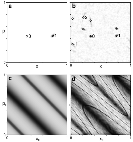
Figure 2: (a) For fixed $\xi_{0}$ the correlator of Husimi amplitudes $c_{1}(\xi_{0};\xi)$ is displayed ($N=1024$). The point $\xi_{0}$ and its classical iterate $\xi_{1}$ are marked by circles. (b) Same for the density correlator $C_{H}(\xi_{0};\xi)$. Labeled circles show the classical trajectory $\xi_{t}$. Unlabeled circles show the time-reversed trajectory $\tilde{\xi}_{t}$ obtained by the transformation (19). (c) $c_{1}(\xi_{0};\xi_{1})$ is shown as a function of $\xi_{0}$. The magnitude of correlation is approximately constant along lines $x_{1}=x_{0}+p_{0}=$ const. (d) Same for $C_{H}(\xi_{0};\xi_{1})$. On top of a background depending on $x_{1}$ one observes smooth fluctuations and relatively sharp lines of excess correlation which correspond to Eq. (20).

It is straightforward to obtain a semiclassical approximation to Eq. (11). Using the completeness of eigenstates we find $\sum_{n}{\rm e}^{+{\rm i}\varepsilon_{n}t/\hbar}h_{n}^{*}(\xi_{0})h_{n}(\xi)=\langle\alpha_{\xi}|\hat{U}^{t}|\alpha_{\xi_{0}}\rangle$. As the semiclassical limit is approached, $\hat{U}^{t}|\alpha_{\xi_{0}}\rangle$ localizes at $\xi_{t}$ and the overlap with $|\alpha_{\xi}\rangle$ vanishes for any other given point (Fig. 2a). Therefore all relevant correlations are given by $c_{t}(\xi_{0};\xi_{t})=|a_{t}(\xi_{0})|^{2}$ with

$$a_{t}(\xi_{0})=\langle\alpha_{\xi_{t}}|\hat{U}^{t}|\alpha_{\xi_{0}}\rangle.$$ (12)

Finally, this overlap is approximated semiclassically with the help of Eqs. (6), (7). For example we find at $t=1$

$$|a_{1}(\xi_{0})|^{2}=2^{3/2}(9+[2V^{\prime\prime}(x_{0}+p_{0})-1]^{2})^{-1/2}.$$ (13)

Note that $c_{1}(\xi_{0};\xi_{1})=|a_{1}(\xi_{0})|^{2}$ depends only on $x_{1}=x_{0}+p_{0}$ which explains the stripes in Fig. 2c. In Fig. 3 we check the accuracy of Eq. (13) by comparing it to the exact value for $N=1024$ (points vs solid line).

Figure 3: Amplitude and density correlators $c_{1}(\xi_{0};\xi_{1})$ (points) and $C_{H}(\xi_{0};\xi_{1})$ (error bars) are compared to the semiclassical prediction Eq. (13) (solid line). An error bar shows mean value and standard deviation of those data from Fig. 2d which are on the line $x_{1}=x_{0}+p_{0}$ but away from the exceptional curves given by Eq. (20).

We continue with a semiclassical theory for the density correlator Eq. (10) which allows to understand the main features observed in Figs. 2b,d. For this purpose we rephrase Eq. (12) as

$$\hat{U}^{t}|\alpha_{0}\rangle=a_{t}|\alpha_{t}\rangle+r_{t}|\rho_{t}\rangle$$ (14)

where $|\rho_{t}\rangle$ is a normalized state which is localized near $\xi_{t}$ but orthogonal to the coherent state at this position, $\langle\rho_{t}|\alpha_{t}\rangle=0$. In other words, $|\alpha_{t}\rangle$ and $|\rho_{t}\rangle$ can be considered as part of some orthonormal basis spanning the Hilbert space. In the spirit of random-matrix theory one can assume that the coefficients of an eigenstate $|n\rangle$ in this basis, and in particular $\alpha_{t,n}\equiv\langle n|\alpha_{t}\rangle$ and $\rho_{t,n}\equiv\langle n|\rho_{t}\rangle$ are uncorrelated,

$$P(\rho_{t,n},\alpha_{t,n})=P(\rho_{t,n})\,P(\alpha_{t,n})\,.$$ (15)

Deferring a discussion of the validity of Eq. (15) we first point out its implications. We multiply the identity

$$H_{0,n} = |\langle n|\hat{U}^{t}|\alpha_{0}\rangle|^{2}$$

$$= |a_{t}|^{2}\,|\alpha_{t,n}|^{2}+2\mbox{Re}\,a^{*}_{t}r_{t}\alpha_{t,n}^{*}\rho_{t,n}+|r_{t}|^{2}|\rho_{t,n}|^{2}$$

with $H_{t,n}=|\alpha_{t,n}|^{2}$ and average over $n$. Then the second term on the r.h.s. vanishes since, according to Eq. (15), the phases from $\alpha_{t,n}^{*}$ and $\rho_{t,n}$ are uncorrelated. Also the third term factorizes and gives $\langle|\alpha_{t,n}|^{2}\rangle_{n}\,|r_{t}|^{2}\langle|\rho_{t,n}|^{2}\rangle_{n}=(1-|a_{t}|^{2})/N^{2}$ after using the normalization implied by Eq. (14). Substitution of these results into Eq. (10) yields after straightforward calculation

$$C_{H}(\xi_{0};\xi_{t}) = |a_{t}|^{2}\sqrt{(N{\cal I}_{t}-1)/(N{\cal I}_{0}-1)}$$ (17)

$$\sim |a_{t}|^{2}\,,$$ (18)

where ${\cal I}_{t}=\sum_{n}H_{t,n}^{2}$ is the inverse participation number in Husimi representation. The approximation ${\cal I}_{0}\sim{\cal I}_{t}$ leading to from (17) to (18) is justified since deviations from the constant ${\cal I}=2/N$ expected within RMT are mainly due to the influence of periodic orbits Heller (1984) which is approximately equal if two points $\xi_{0}$ and $\xi_{t}$ connected by a short trajectory.

Eq. (18) suggests that also $C_{H}(\xi_{0};\xi_{1})$ is given by Eq. (13). This is confirmed by the data in Figs. 2d and 3 (error bars vs solid line) if the conspicuous sharp curves of very large correlation (Fig. 2d) are ignored. To understand the origin of such exceptional points where the above theory fails we return now to the crucial step in the derivation, Eq. (15). A RMT assumption like this is justified only after all important non-generic effects have been accounted for. These include in particular symmetries and semiclassical contributions from short trajectories. Hence, as $|\alpha_{t}\rangle$ and $|\rho_{t}\rangle$ are both concentrated near $\xi_{t}$, we expect that Eq. (15) breaks down whenever this point is on a symmetry line or on a periodic orbit. For example, if $\xi_{0}=\xi_{t}$ we have obviously $C_{H}(\xi_{0};\xi_{t})=1$ but $|a_{t}|^{2}\ll 1$ if the orbit is sufficiently unstable. In our model the only symmetry is time reversal: the unitary transformation $\tilde{U}=D^{\dagger}UD$ with $D=\exp(-{\rm i}V/2\hbar)$ leads to a symmetric propagator $\tilde{U}=\tilde{U}^{T}$. As a consequence the eigenfunctions of $\tilde{U}$ are real in position representation and their Husimi density is symmetric with respect to $p=0$. After back transformation to the original basis we infer from this symmetry that the Husimi density at $\xi$ is correlated with the density at

$$\tilde{\xi}=(x,-p-V^{\prime}(x))$$ (19)

which is confirmed in Fig. 2b. For the torus map Eq. (2) the point $\xi_{t}$ is invariant under this transformation if $[2p_{t}+V^{\prime}(x_{t})]\,\mbox{mod}\,1=0$. Indeed we obtain from this condition with $t=1$ the correct functional equation for the lines of excess correlation in Fig. 2d,

$$[2p_{0}-V^{\prime}(x_{0}+p_{0})]\,\mbox{mod}\,1 = 0.$$ (20)

Note that short periodic orbits of period $1$ and $2$ must be invariant under time reversal and are located on these lines. In other numerical data for maps without time-reversal invariance we found excess correlations only at isolated points corresponding to the short orbits. A quantitative and more detailed analysis of excess correlations is still to be done. We expect that this will be feasible by applying Gaussian wavepacket dynamics again, now in order to correlate the states $|\alpha_{t}\rangle$ and $|\rho_{t}\rangle$ semiclassically.

We end this paper with a remark on the parameter $|a_{t}|^{2}$ which essentially determines the Husimi correlations. Fig. 3 shows that it can be very large even in a completely chaotic system. In fact $|a_{1}|^{2}$ (Eq. (13)) is not directly related to the local stability eigenvalues of the classical map. As explained after Eq. (7), this changes only when the width of the Gaussian is much larger than that of a coherent state, i.e., when $|a_{t}|^{2}$ is already very small.