Quantifying Self-Organization with Optimal Predictors

Abstract

Despite broad interest in self-organizing systems, there are few quantitative, experimentally-applicable criteria for self-organization. The existing criteria all give counter-intuitive results for important cases. In this Letter, we propose a new criterion, namely an internally-generated increase in the statistical complexity, the amount of information required for optimal prediction of the system’s dynamics. We precisely define this complexity for spatially-extended dynamical systems, using the probabilistic ideas of mutual information and minimal sufficient statistics. This leads to a general method for predicting such systems, and a simple algorithm for estimating statistical complexity. The results of applying this algorithm to a class of models of excitable media (cyclic cellular automata) strongly support our proposal.

The term “self-organization” was coined in the 1940s Ashby (1947) to label processes in which systems become more highly organized over time, without being ordered by outside agents or by external programs. It has become one of the leading concepts of nonlinear science, without ever having been properly defined. The prevailing “I know it when I see it” standard prevents the development of a theory of self-organization. Thus some say that “self-organizing” implies “dissipative” Nicolis and Prigogine (1977), and others that they can exhibit reversible self-organization D’Souza and Margolus (1999); Smith (2003), and no one knows if both groups are talking about the same idea.

A definition of self-organization should be mathematically precise, so we can build theories around it, and experimentally applicable, so we can use empirical data to say whether something self-organizes. The goal of such a definition should be both to match our informal notions in easy cases, where intuition is clear and consensual, and to extend unambiguously to intuitively hard or disputed cases. If our informal notions allow for comparative, “more than” judgments, a formalization should match those, too. Generally there are many ways to formalize a single concept, and competing formalizations must be judged by their scientific fruitfulness; differing formalizations may be appropriate in different contexts. (For more on such methodological issues, see Quine (1961).)

We believe we have a formal criterion for self-organization that meets the key requirements. It is precise, unambiguous, and operational. We check its conformity with intuition against cellular automata, specifically cyclic cellular automata (CA). They are ideal test cases: their dynamics are completely known (because we specify them) and can easily be simulated exactly. They are reasonable qualitative models of excitable media, and there is an analytical theory Fisch et al. (1991) of the patterns they form. We show that our definition works, at least in this case. Two of us discussed preliminary work in Shalizi and Shalizi (2003); here we present the (concurring) results of larger, more extensive simulations.

Measuring Organization Few attempts have been made to measure self-organization quantitatively. Thermodynamic entropy is an obvious measure of organization for physicists, and several works claim to measure self-organization by finding spontaneous declines in entropy Wolfram (1983); Krepeau and Isaacson (1990); Klimontovich (1991). But thermodynamic entropy is a bad measure of organization in complex systems Fox (1988); Sewell (2002); Badii and Politi (1997). Entropy is proportional to the logarithm of the accessible volume in phase space, which has no necessary connection to any kind of organization. Thus low-temperature states of Ising systems or Fermi fluids have very low entropy, but no discernible organization Sewell (2002). Biological organisms are never in pure, low-entropy states, but are organized, if anything is. Some kinds of biological self-organization are, in fact, thermodynamically driven by increasing entropy Fox (1988); Privalov and Gill (1988).

After “fall in entropy”, the leading idea on how to measure self-organization, advanced in Bennett (1985), is a rise in complexity. While there are many proposed measures of physical complexity, the general view is that complex phenomena are ones which cannot be described concisely and accurately (see Badii and Politi (1997) for a general survey). Most proposals use algorithmic descriptions, and are limited by inherent uncomputability. Here we take a stochastic point of view, aiming to statistically describe ensembles of configurations. We follow Grassberger Grassberger (1986) in defining the complexity of a process as the least amount of information about its state needed for maximally accurate prediction. Crutchfield and Young Crutchfield and Young (1989) extended this concept, by giving operational definitions of “maximally accurate prediction” and “state”.

The Grassberger-Crutchfield-Young “statistical complexity”, $C$, is the information content of the minimal sufficient statistic for predicting the process’s future Shalizi and Crutchfield (2001). In thermodynamic settings, this is the amount of information a full set of macrovariables contains about the system’s microscopic state Shalizi and Moore (2003). We now sketch the formalism allowing us to use statistical complexity to characterize spatially-extended dynamical systems of arbitrary dimension, after Shalizi (2003).

Let $x(\vec{r},t)$ be an $n+1$D field, possibly stochastic, in which interactions between different space-time points propagate at speed $c$. As in Parlitz and Merkwirth (2000), define the past light cone of the space-time point $(\vec{r},t)$ as all points which could influence $x(\vec{r},t)$, i.e., all points $(\vec{q},u)$ where $u<t$ and $||\vec{q}-\vec{r}||\leq c(t-u)$. The future light cone of $(\vec{r},t)$ is the set of all points which could be influenced by what happens at $(\vec{r},t)$. $l^{-}(\vec{r},t)$ is the configuration of the field in the past light cone, and ${l}^{+}(\vec{r},t)$ the same for the future light cone. The distribution of future light cone configurations, given the configuration in the past, is ${\rm P}({l}^{+}|l^{-})$.

Any function $\eta$ of $l^{-}$ defines a local statistic. It summarizes the influence of all the space-time points which could affect what happens at $(\vec{r},t)$. Such local statistics should tell us something about “what comes next,” which is ${l}^{+}$. (Shalizi (2003) explains why we must use local predictors, and the advantages of basing them on light cones, as first suggested by Parlitz and Merkwirth (2000).) Information theory lets us quantify how informative different statistics are.

The information about variable $x$ in variable $y$ is $I[x;y]$,

$$I[x;y] \equiv \left\langle\log_{2}{\frac{{\rm P}(x,y)}{{\rm P}(x){\rm P}(y)}}\right\rangle$$ (1)

where ${\rm P}(x,y)$ is joint probability, ${\rm P}(x)$ is marginal probability, and $\langle\cdot\rangle$ is expectation Kullback (1959). The information a statistic $\eta$ conveys about the future is $I[{l}^{+};\eta(l^{-})]$. A statistic is sufficient if it is as informative as possible Kullback (1959), here if and only if $I[{l}^{+};\eta(l^{-})]=I[{l}^{+};l^{-}]$. This is the same Kullback (1959) as requiring that ${\rm P}({l}^{+}|\eta(l^{-}))={\rm P}({l}^{+}|l^{-})$. A sufficient statistic retains all the predictive information in the data. Decision theory Blackwell and Girshick (1954) tells us that maximally accurate and precise prediction needs only a sufficient statistic, not the original data; in fact, any predictor which does not use a sufficient statistic can be replaced by a superior one which does. Since we want optimal prediction, we confine ourselves to sufficient statistics.

If we use a sufficient statistic $\eta$ for prediction, we must describe or encode it. Since $\eta(l^{-})$ is a function of $l^{-}$, this encoding takes $I[\eta(l^{-});l^{-}]$ bits. If knowing $\eta_{1}$ lets us compute $\eta_{2}$, which is also sufficient, then $\eta_{2}$ is a more concise summary, and $I[\eta_{1}(l^{-});l^{-}]\geq I[\eta_{2}(l^{-});l^{-}]$. A minimal sufficient statistic Kullback (1959) can be computed from any other sufficient statistic. We now construct one.

Take two past light cone configurations, $l^{-}_{1}$ and $l^{-}_{2}$. Each has some conditional distribution over future light cone configurations, ${\rm P}({l}^{+}|l^{-}_{1})$ and ${\rm P}({l}^{+}|l^{-}_{2})$ respectively. The two past configurations are equivalent, $l^{-}_{1}\sim l^{-}_{2}$, if those conditional distributions are equal. The set of configurations equivalent to $l^{-}$ is $[l^{-}]$. Our statistic is the function which maps past configurations to their equivalence classes:

$$\epsilon(l^{-})\equiv[l^{-}]=\left\{\lambda~{}:~{}{\rm P}({l}^{+}|\lambda)={\rm P}({l}^{+}|l^{-})\right\}$$ (2)

Clearly, ${\rm P}({l}^{+}|\epsilon(l^{-}))={\rm P}({l}^{+}|l^{-})$, and so $I[{l}^{+};\epsilon(l^{-})]=I[{l}^{+};l^{-}]$, making $\epsilon$ a sufficient statistic. The equivalence classes, the values $\epsilon$ can take, are the causal states Shalizi (2003); Crutchfield and Young (1989); Shalizi and Crutchfield (2001); Shalizi and Moore (2003). Each causal state is a set of specific past light-cones, and all the cones it contains are equivalent, predicting the same possible futures with the same probabilities. Thus there is no advantage to subdividing the causal states, which are the coarsest set of predictively sufficient states.

For any sufficient statistic $\eta$, ${\rm P}({l}^{+}|l^{-})={\rm P}({l}^{+}|\eta(l^{-}))$. So if $\eta(l^{-}_{1})=\eta(l^{-}_{2})$, then ${\rm P}({l}^{+}|l^{-}_{1})={\rm P}({l}^{+}|l^{-}_{2})$, and the two pasts belong to the same causal state. Since we can get the causal state from $\eta(l^{-})$, we can use the latter to compute $\epsilon(l^{-})$. Thus, $\epsilon$ is minimal. Moreover, $\epsilon$ is the unique minimal sufficient statistic Shalizi (2003): any other just relabels the same states.

Because $\epsilon$ is minimal, $I[\epsilon(l^{-});l^{-}]\leq I[\eta(l^{-});l^{-}]$, for any other sufficient statistic $\eta$. Thus we can speak objectively about the minimal amount of information needed to predict the system, which is how much information about the past of the system is relevant to predicting its own dynamics. This quantity, $I[\epsilon(l^{-});l^{-}]$, is a characteristic of the system, and not of any particular model. We define the statistical complexity as

$$C \equiv I[\epsilon(l^{-});l^{-}]$$ (3)

$C$ is the amount of information required to describe the behavior at that point, and equals the log of the effective number of causal states, i.e., of different distributions for the future. Complexity lies between disorder and order Badii and Politi (1997); Grassberger (1986); Crutchfield and Young (1989), and $C=0$ both when the field is completely disordered (all values of $x$ are independent) and completely ordered ($x$ is constant). $C$ grows when the field’s dynamics become more flexible and intricate, and more information is needed to describe the behavior.

We now sketch an algorithm to recover the causal states from data, and so estimate $C$. (Shalizi (2003) provides details, including pseudocode; cf. Parlitz and Merkwirth (2000).) At each time $t$, list the observed past and future light-cone configurations, and put the observed past configurations in some arbitrary order, $\left\{l^{-}_{i}\right\}$. (In practice, we must limit how far light-cones extend into the past or future.) For each past configuration $l^{-}_{i}$, estimate ${\rm P}_{t}({l}^{+}|l^{-}_{i})$. We want to estimate the states, which ideally are groups of past cones with the same conditional distribution over future cone configurations. Not knowing the conditional distributions a priori, we must estimate them from data, and with finitely many samples, such estimates always have some error. Thus, we approximate the true causal states by clusters of past light-cones with similar distributions over future light-cones; the conditional distribution for a cluster is the weighted mean of those of its constituent past cones. Start by assigning the first past, $l^{-}_{1}$ to the first cluster. Thereafter, for each $l^{-}_{i}$, go down the list of existing clusters and check whether ${\rm P}_{t}({l}^{+}|l^{-}_{i})$ differs significantly from each cluster’s distribution, as determined by a fixed-size $\chi^{2}$ test. (We used $\alpha=0.05$ in our simulations below.) If the discrepancy is insignificant, add $l^{-}_{i}$ to the first matching cluster, updating the latter’s distribution. Make a new cluster if $l^{-}_{i}$ does not match any existing cluster. Continue until every $l^{-}_{i}$ is assigned to some cluster. The clusters are then the estimated causal states at time $t$. Finally, obtain the probabilities of the different causal states from the empirical probabilities of their constituent past configurations, and calculate $C(t)$. This procedure converges on the correct causal states as it gets more data, independent of the order of presentation of the past light-cones, the ordering of the clusters, or the size $\alpha$ of the significance test Shalizi (2003). For finite data, the order of presentation matters, but we finesse this by randomizing the order.

We say a system has organized between times $t_{1}$ and $t_{2}$ if (I) $C(t_{2})-C(t_{1})\equiv\Delta C>0$. It has self-organized if (II) some of the rise in complexity is not due to external agents. We can check condition (I) by estimating $\Delta C$. We know condition (II) holds for many systems, because they either have no external inputs (e.g., deterministic CA), or only unstructured inputs (e.g., chemical pattern-formers exposed to thermal noise). For systems with structured input, we need, but lack, a way to say how much of $\Delta C$ is due to that input. We could, perhaps, treat this as a causal inference problem Pearl (2000), with $\Delta C$ as the response variable, and the input as the treatment. Alternately, we could see how much $\Delta C$ changes if we replace the input with statistically-similar noise Delgado and Solé (1997).

Numerical Experiments and Results Having developed a quantitative criterion for self-organization, we now check it experimentally. Our test systems are cyclic cellular automata Fisch et al. (1991) (CCA), which are models of pattern formation in excitable media Tyson and Keener (1988). Each site in a square lattice has one of $\kappa$ colors. A cell of color $k$ will change its color to $k+1\bmod\kappa$ if there are already at least $T$ (“threshold”) cells of that color in its neighborhood, i.e., within a distance $r$ (“range”) of that cell. Otherwise, the cell keeps its current color. (In normal excitable media, which have a unique quiescent state, the role of the threshold is slightly different Tyson and Keener (1988).) All cells update their colors in parallel.

(a) (b)

(c) (d)

Figure 1: (Color online.) Phases of the cyclic CA. Parameters are as described in the text, started from uniform random initial conditions. Color figures were prepared with Wójtowicz (2002). From the top left: (a) Local oscillations $(T=1)$, in which the CA oscillates with period 4, each cell cycling through all colors; (b) Spiral waves $(T=2)$; (c) The “turbulent” phase $(T=3)$; (d) Fixation with solid color blocks $(T=4)$.

CCA have three generic long-run behaviors, depending on the ratio of the threshold to the range. At high thresholds, CCA form homogeneous blocks of solid colors, which are completely static (“fixation”). At very low thresholds, the entire lattice eventually oscillates periodically; sometimes rotating spiral waves grow to engulf the entire lattice. With intermediate thresholds, incoherent traveling waves form, propagate, collide and disperse; this, metaphorically, is “turbulence”. With a range one Moore (box) neighborhood and $\kappa=4$, the phenomenology is as follows Fisch et al. (1991) (see Fig. 1). $T=1$ and $T=2$ are both locally periodic, but $T=2$ produces spiral waves, while $T=1$ quenches incoherent local oscillations. $T=3$ leads to meta-stable turbulence — spiral waves can form and entrain the entire CA, but turbulence can persist indefinitely on finite lattices. Fixation occurs with $T\geq 4$. All CCA phases self-organize when started from uniform noise. (This is best appreciated by viewing simulations Wójtowicz (2002).) By the same intuitive standard, the fixation phase is less organized than turbulence (which has dynamic, large-scale spatial structures), which in turn is less organized than spiral waves (which has more intricate structures). It is hard to say, by eye, whether incoherent local oscillations are more or less organized than simple fixation. All four regimes lead to stable stationary distributions. Thus, $C$ should start at zero (reflecting the totally random initial conditions), rise to a steady value, and stay there. $T=2$ should have the highest long-run complexity, followed by $T=3$.

We ran $\kappa=4$, $r=1$ CCA on $300\times 300$ lattices with periodic boundary conditions, for $T$ from 1 to 4. Figure 2 shows the results of applying our proposed measure of self-organization to these simulations. We used light-cones extending 1 time-step into both past and future; longer light-cones did not, here, lead to different states. The agreement with expectations is clear. All four curves climb steadily to plateaus, leveling off when the distribution of CA configurations become stationary. Sampling noise leads to fluctuations around the asymptotic values Shalizi and Shalizi (2003). The slight fall in complexity for $T=3$ occurs when spirals try to form but break up, and their debris limit further spiral formation. Additional simulations at different lattice sizes $L$ show the estimated long-run complexity growing with $L$, approaching a limit as $O(L^{-1})$. This rate combines finite-size effects with the negative bias of our information estimator, which is at least $O(L^{-2})$ Victor (2000). We hope in the future to precisely determine both our estimation bias and the finite-size scaling of the complexity.

Conclusion A theory of self-organization should predict when and why different systems will assume different kinds and degrees of organization. This will require an adequate characterization of self-organization. We argue that “internally-caused rise in complexity” works, if we define complexity as the amount of information needed for optimal statistical prediction. We can reliably estimate this statistical complexity from data, and for CCA, the estimates match intuitive judgments about self-organization. The methods used are not limited to CA, but apply to all kinds of discrete random fields, including ones on complex networks Shalizi (2003). They would work equally well on discretized empirical data, e.g., digital movies of chemical pattern formation experiments. This is a first step towards a physical theory of self-organization.

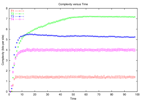
Figure 2: (Color online.) Complexity over time for CCA with different thresholds $T$, averaging 30 independent simulations at each value of $T$. The $T=2$ curve has the highest asymptote, followed by $T=3$, $T=4$ and $T=1$. Error bars: standard error of the complexity.

Acknowledgments We thank D. Abbott, J. Crutchfield, R. D’Souza, D. Feldman, D. Griffeath, C. Moore, S. Page, M. Porter, E. Smith, J. Usinowicz and our referees.

References

- Ashby (1947) W. R. Ashby, J. General Psychology 37, 125 (1947).
- Nicolis and Prigogine (1977) G. Nicolis and I. Prigogine, Self-Organization in Nonequilibrium Systems (Wiley, New York, 1977).
- D’Souza and Margolus (1999) R. M. D’Souza and N. H. Margolus, Phys. Rev. E 60, 264 (1999), URL cond-mat/9810258.
- Smith (2003) E. Smith, Phys. Rev. E 68, 046114 (2003).
- Quine (1961) W. V. O. Quine, From a Logical Point of View (Harvard U. P., Cambridge, Mass., 1953).
- Fisch et al. (1991) R. Fisch, J. Gravner, and D. Griffeath, Stat. Comput. 1, 23 (1991), URL psoup.math.wisc.edu/papers/tr.zip.
- Shalizi and Shalizi (2003) C. R. Shalizi and K. L. Shalizi, in Noise in Complex Systems and Stochastic Dynamics, edited by L. Schimansky-Geier et al. (SPIE, Bellingham, Washington, 2003), pp. 108–117, URL bactra.org/research/FN03.pdf.
- Bak et al. (1987) P. Bak, C. Tang, and K. Wiesenfeld, Phys. Rev. Lett. 59, 381 (1987).
- Wolfram (1983) S. Wolfram, Rev. Mod. Phys. 55, 601 (1983).
- Krepeau and Isaacson (1990) J. C. Krepeau and L. K. Isaacson, J. Noneq. Thermo. 15, 115 (1990).
- Klimontovich (1991) Y. L. Klimontovich, Turbulent Motion and the Structure of Chaos (Kluwer, Dordrecht, 1991).
- Fox (1988) R. F. Fox, Energy and the Evolution of Life (Freeman, New York, 1988).
- Sewell (2002) G. L. Sewell, Quantum Mechanics and Its Emergent Macrophysics (Princeton U. P., Princeton, 2002).
- Badii and Politi (1997) R. Badii and A. Politi, Complexity: Hierarchical Structures and Scaling in Physics (Cambridge U. P., Cambridge, 1997).
- Privalov and Gill (1988) P. L. Privalov and S. J. Gill, Adv. Protein Chem. 39, 191 (1988).
- Bennett (1985) C. H. Bennett, in Emerging Syntheses in Science, edited by D. Pines (Santa Fe Institute, Santa Fe, New Mexico, 1985), pp. 215–234.
- Grassberger (1986) P. Grassberger, Int. J. Theor. Phys. 25, 907 (1986).
- Crutchfield and Young (1989) J. P. Crutchfield and K. Young, Phys. Rev. Lett. 63, 105 (1989).
- Shalizi and Crutchfield (2001) C. R. Shalizi and J. P. Crutchfield, J. Stat. Phys. 104, 817 (2001), URL cond-mat/9907176.
- Shalizi and Moore (2003) C. R. Shalizi and C. Moore, Studies Hist. Phil. Mod. Phys. submitted (2003), URL cond-mat/0303625.
- Shalizi (2003) C. R. Shalizi, Discrete Math. Theor. Comput. Sci. AB(DMCS), 11 (2003), URL math.PR/0305160.
- Parlitz and Merkwirth (2000) U. Parlitz and C. Merkwirth, Phys. Rev. Lett. 84, 1890 (2000).
- Kullback (1959) S. Kullback, Information Theory and Statistics (Wiley, New York, 1959).
- Blackwell and Girshick (1954) D. Blackwell and M. A. Girshick, Theory of Games and Statistical Decisions (Wiley, New York, 1954).
- Pearl (2000) J. Pearl, Causality: Models, Reasoning, and Inference (Cambridge U. P., Cambridge, 2000).
- Delgado and Solé (1997) J. Delgado and R. V. Solé, Physical Review E 55, 2338 (1997).
- Tyson and Keener (1988) J. J. Tyson and J. P. Keener, Physica D 32, 327 (1988).
- Wójtowicz (2002) M. Wójtowicz, Cellebration, Online software (2002), URL psoup.math.wisc.edu/mcell/.
- Victor (2000) J. D. Victor, Neural Computation 12, 2797 (2000).