Resonant light scattering by optical solitons

Abstract

We consider the process of light scattering by optical solitons in a planar waveguide with homogeneous and inhomogeneous refractive index core. We observe resonant reflection (Fano resonances) as well as resonant transmission of light by optical solitons. All resonant effects can be controlled in experiment by changing the soliton intensity.

Recently the problem of plane wave scattering by various time-periodic potentials has attracted much attention, as it has been shown that some interesting effects such as resonant reflection of waves Cretegny can be observed when dealing with non-stationary scattering centers. These resonant reflection effects were demonstrated to be similar to the well-known Fano resonance Fano for some nonlinear systems Flach . In one-dimensional (1D) systems they can lead to the total resonant reflection of waves. The time-periodic scattering centers can originate from the presence of nonlinearity in a spatially homogeneous system DB-REVIEWS . The main underlying idea of this phenomenon is that a nonlinear time-periodic scattering potential induces several harmonics. In general, these harmonics can be either inside or outside the plane wave spectrum, ’open’ and ’closed’ channels, respectively Flach . The presence of closed channels is equivalent to a local increase of the spatial dimensionality, i.e. to the appearance of alternative paths for the plane wave to propagate. This can lead to novel interference effects, such as the resonant reflection of waves - Fano resonance in nonlinear systems.

Here we emphasize, that the total resonant reflection of plane waves can be similarly arranged by means of a static scattering center, provided the system dimensionality has been artificially locally increased (e.g. in composite materials) Fano_stac . However, such static configurations have at least two significant disadvantages. Firstly, they do not provide any flexibility in tuning the resonance parameters: the resonant values of plane wave parameters are fixed by the specific geometry. Secondly, it may be a nontrivial technological task to introduce locally additional degrees of freedom for plane waves in the otherwise 1D system. Time-periodic scattering potentials appear to be much more promising: they can be relatively easily generated (e.g. laser beams, microwave radiation, localized soliton-like excitations), and they provide us with an opportunity to tune the resonance, since all the resonant parameters are depending on the parameters of the potential (e.g. amplitude, frequency) and thus can be ’dynamically’ controlled by some parameter, e.g. the laser beam intensity.

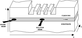
Figure 1: Schematic structure of the experimental setup. The soliton beam is sent along the $z$-axis, while the ’probe’ beam propagates in the $xz$-plane at some angle to the soliton.

In this Letter we demonstrate a possibility of experimental observation of Fano resonances in the scattering process of light by optical spatial solitons. The soliton is generated in a planar (slab) waveguide by a laser beam injected into the slab along the $z$-direction, see Fig. 1. The soliton beam light is confined in the $y$-direction (inside the core layer) by the total internal reflection. The localization of light in the $x$-direction (the spatial soliton propagates along the $z$-direction) is ensured by the balance between linear diffraction and an instantaneous Kerr-type nonlinearity. The probe beam is sent at some angle to the soliton. It has small enough amplitude so that the Kerr nonlinearity of the medium is negligible outside the soliton core. It is important to note, that the process of light scattering by a spatial soliton is assumed to be stationary in time, i.e. the light is quasi-monochromatic. The analogy with the above time-periodic scattering problems comes from the possibility to interpret the spatial propagation along the $z$-direction as an artificial time Zaharov ; Agrawal . Thus the angle, at which the probe beam is sent to $z$-axis plays the role of a parameter similar to the frequency (or wave number) of plane waves in 1D systems.

In addition we allow the refractive index $n$ inside the slab to be a stepwise function of the coordinate $x$ in a finite region, where the soliton is located, and $n(x)\equiv n_{0}$ elsewhere. The modulation of the refractive index can be achieved by means of well-established techniques of producing waveguide arrays: either by etching the surface of the waveguide Eisenberg , or by inserting stripes of another material into the slab Shimshon .

Assuming that the electromagnetic field maintains its linear polarization, the stationary Maxwell equation for the Fourier component of the electric field $E(x,z)$ footnote takes the following form Ablowitz_Musslimani :

$$\frac{\partial^{2}E}{\partial z^{2}}+\frac{\partial^{2}E}{\partial x^{2}}+n^{2}(x)E+\alpha\left|E\right|^{2}E=0,$$ (1)

where $\alpha>0$ is the nonlinear Kerr coefficient, the electromagnetic field is considered to be monochromatic $\mathcal{E}(x,z,t)=E(x,z)\exp(-i\omega t)+c.c.$, and the dimensionless spatial coordinates are used: $\omega/c=1$, with $c$ being speed of light in vacuum.

A spatial optical soliton represents a special class of solutions of Eq.(1) of the form $E^{sol}(x,z)=C(x)\exp(i\beta z)$ with $C(x)$ describing the exponentially localized profile of the soliton, $C(x)|_{x\rightarrow\pm\infty}\rightarrow 0$. $\beta$ is the only soliton parameter ($z$-component of its wave-vector), $\beta>n_{0}$. The soliton envelope function $C(x)$ satisfies the stationary nonlinear Schrödinger equation (NLS):

$$\frac{d^{2}C}{dx^{2}}+\left[n^{2}(x)-\beta^{2}\right]C+\alpha\left|C\right|^{2}C=0,$$ (2)

The probe beam light interacts with the optical soliton, so that the total electric field is a sum of two contributions, $E(x,z)=L(x,z)+C(x)\exp(i\beta z)$, both ideally having the same frequency $\omega$. Treating the probe beam part $L$ as a small perturbation to the soliton part $C$ allows for a linearization of Eq.(1) around the soliton solution, so that we obtain:

$$\frac{\partial^{2}L}{\partial z^{2}}+\frac{\partial^{2}L}{\partial x^{2}}+n^{2}(x)L+\alpha\left[2|C|^{2}L+\mu L^{*}C^{2}e^{i2\beta z}\right]=0.$$ (3)

The soliton acts as an external potential for the linear beam, consisting of a ’DC’ ($\sim|C|^{2}$) and ’AC’ ($\sim C^{2}$) parts. While the former is the soliton induced nonlinear refractive index modulation, the latter is the result of a coherent interaction between the beams. Thus, the ratio of AC/DC components depends on the coherence level between the soliton and the probe beam, which can be controlled in experiment e.g. by a slight beam frequency detuning or by changing the spatial correlation length between them. The effective parameter $\mu$ ($0\leq\mu\leq 1$) accounts for this possible decoherence between the beams.

The soliton part is negligible, $C(x)\rightarrow 0$, outside the scattering center and the refractive index is constant $n(x)\equiv n_{0}$. Then Eq.(3) reduces to the simple wave equation for plane waves $L(x,z)\sim\exp(ik_{x}x+ik_{z}z)$ with the dispersion relation:

$$k_{x}^{2}+k_{z}^{2}=n_{0}^{2}.$$ (4)

Both the modulation of the refractive index and the soliton (the DC part of the corresponding potential to be more precise) can result in bound states for the probe light with the wave vector components $(k_{x},k_{z})$ lying outside the spectrum (4). Besides, the soliton acts as a harmonic generator (via its AC part), so that the general solution of the eq.(3) consists of two ”harmonics” (two channels):

$$L(x,z)=A(x)\exp[ik_{z}z]+B(x)\exp[i(2\beta-k_{z})z],$$ (5)

coupled to each other via the AC part of the soliton scattering potential Flach :

$$A^{\prime\prime}=\left[k_{z}^{2}-n^{2}(x)\right]A-\alpha\left[2|C|^{2}A+\mu B^{*}C^{2}\right],$$ (6)

$$B^{\prime\prime}=\left[(2\beta-k_{z})^{2}-n^{2}(x)\right]B-\alpha\left[2|C|^{2}B+\mu A^{*}C^{2}\right].$$ (7)

For zero coherence parameter, $\mu=0$, the equation for $A$ ($B$) channel is equivalent to the stationary Schrödinger equation for an effective particle with the energy $E_{A}=n_{0}^{2}-k_{z}^{2}$ ($E_{B}=n_{0}^{2}-(2\beta-k_{z})^{2}$) in the external potential being the sum of ’geometrical’ and ’soliton’ parts: $V_{eff}(x)=[n_{0}^{2}-n^{2}(x)]-2\alpha|C(x)|^{2}$.

We chose $0\leq k_{z}\leq n_{0}$, so that it satisfies the dispersion relation (4) with a real $k_{x}$ value and the probe beam wave can freely propagate far away from the scattering center. Thus the $z$-component of the wave vector in the second term in (5) $2\beta-k_{z}$ is outside the spectrum (4). This term corresponds to a closed channel with amplitude exponentially decaying with the increasing distance from the scattering center. Hence, we have one open ($A$) and one closed ($B$) channel in our scattering problem.

There is a limiting case when we can predict the position of a Fano resonance. It corresponds to a small coupling between the two channels provided by the AC scattering potential. Then the Fano resonance is located at the resonance between the discrete part of the closed channel spectrum (localized states) and the continuum part of the open channel spectrum (delocalized states). We take advantage of this limit by choosing the coherence parameter $\mu$ to be small, $\mu\rightarrow 0$ (incoherent interaction). We will use this limit as the starting point to catch the resonance and to follow it while increasing the AC potential strength to its proper value for the coherent interaction, $\mu\rightarrow 1$. By subsequently increasing the coupling between the open and closed channels, we strongly affect the position of localized levels in spectra of these channels. Therefore even a weak modulation of the refractive index $n$, which also affects the positions of localized levels, might play an important role in the process of light scattering by optical solitons.

To compute the transmission coefficient $T(k_{x})$ we solve eqs. (6,7) with the boundary conditions Flach : $A(x\rightarrow+\infty)=\tau\exp(ik_{x}x)$, $A(x\rightarrow-\infty)=\exp(ik_{x}x)+\rho\exp(-ik_{x}x)$, $B(x\rightarrow+\infty)=F\exp(-\kappa x)$, $B(x\rightarrow-\infty)=D\exp(\kappa x)$. Amplitudes of transmitted, $\tau$, and reflected, $\rho$, waves in the open channel define the transmission and reflection coefficients: $T=|\tau|^{2}=1-|\rho|^{2}=1-R$, respectively. Amplitudes $F$ and $D$ describe spatially exponentially decaying closed channel excitations with the inverse localization length $\kappa=[4\beta^{2}-4\beta\sqrt{n_{0}^{2}-k_{x}^{2}}-k_{x}^{2}]^{0.5}$.

In the simplest case of a homogeneous planar waveguide core $n(x)\equiv n_{0}=const.$ $C(x)$ is the well-known stationary NLS soliton Zaharov :

$$C(x)=\sqrt{\frac{2\left(\beta^{2}-n_{0}^{2}\right)}{\alpha}}\frac{1}{\cosh\left[\sqrt{\beta^{2}-n_{0}^{2}}x\right]}$$ (8)

All resonance effects are suppressed in the fully coherent case ($\mu=1$) due to the transparency of the NLS soliton Zaharov , see Fig. 2, even though the resonance condition described above can be formally satisfied for the soliton parameter $\beta$ lying in the interval $1<\beta/n_{0}\lessapprox 1.5$. However, at small $\mu$ we observe the Fano resonance at wavenumbers $k_{x}$ close to the predicted position in the limit of a small interchannel coupling (dependent on the soliton parameter $\beta$), see Fig. 2. Increasing coherency $\mu$ leads to a shift of the resonance position towards the band edge $k_{x}=0$ (this limiting value corresponds to the ’probe’ beam being sent along the $z$-axis, i.e. parallel to the soliton). Finally, when the soliton and the probe beam are coherent ($\mu=1$), we loose the resonance completely and the soliton becomes transparent ($T\equiv 1$).

In order to observe Fano resonances for coherent beams we consider a non-homogeneous refractive index $n(x)$. Introducing modulation of the refractive index, the soliton is no longer transparent for the probe beam. However, this does not automatically guarantee appearance of resonances, thus specific core configurations must be designed.

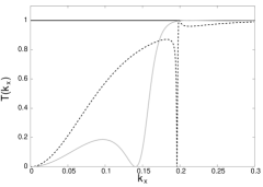
Figure 2: Transmission coefficient $T(k_{x})$ of the probe beam through the optical soliton with $\beta\approx 1.4743$, $\beta^{2}-n_{0}^{2}=0.1$, in the case of a homogeneous core of the planar waveguide with $n_{0}=1.44$ (solid black line). The dashed and solid gray lines indicate the transmission coefficient for the same system but for partially decoherent beams with $\mu=0.1$ and $\mu=0.5$, respectively.

We propose here a triple well (TW) configuration of the planar waveguide core, which allows one to observe the Fano resonance effect in light scattering by an optical soliton. The refractive index $n(x)$ inside the core is locally decreased in the vicinity of the scattering center (i.e. where an optical soliton is formed), $n(x)=n_{1}<n_{0},|x|<L$. In addition, to stabilize the soliton, we introduce local ’wells’ with a higher value of the refractive index $n=n_{2}$ ($n_{1}<n_{2}<n_{0}$) inside the $n=n_{1}$ section, the width of each well is $L_{b}<L$. It would suffice to insert only one well, but the TW configuration provides one with more pronounced Fano resonances. The resulting structure of the effective potential $n_{0}^{2}-n^{2}(x)$, caused by the refractive index modulation, and the stable optical soliton profile $C(x)$ are shown in Fig. 3(a). The transmission coefficient computed for the system both with and without solitons with different parameters is plotted in Fig. 3(b).

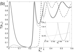
Figure 3: (a) The effective potential $n_{0}^{2}-n^{2}(x)$ (dashed line) and the soliton profile $C(x)$ (solid line) for the TW configuration, parameter values are: $n_{0}=1.44$, $n_{1}=1.4$, $n_{2}=1.42$, $L=12$, $L_{b}=4$, $\beta\approx 1.4417$, $\beta^{2}-n_{0}^{2}=5.0e$-3. The dotted line shows the soliton profile for the case of a homogeneous core $n(x)\equiv n_{0}=1.44$ with the same value of the soliton parameter $\beta$; (b) Transmission coefficient $T(k_{x})$ for the system without a soliton (dashed line), and with solitons having different parameter values: $\beta\approx 1.4417$, $\beta^{2}-n_{0}^{2}=5.0e$-3 (solid black line), $\beta\approx 1.4434$, $\beta^{2}-n_{0}^{2}=1.0e$-2 (solid gray line). Vertical line indicates the critical value $\hat{k}\approx 0.337$ (see the main text for details). Note, that $\mu=1$ here (coherent interaction).

Note, that the $T(k_{x})$ dependence for the TW configuration without a soliton has several peculiarities. First of all, there is always a critical value $\hat{k}$, below which the transmission coefficient is rather small. This has a direct connection to the well known effect of the ’total internal reflection’ at the boundary between the homogeneous core and the central section with a lower value of the refractive index. In addition, we observe several transmission peaks at larger $k_{x}$ values connected with internal modes and determined by the specific internal configuration of the TW section [i.e. by the $n(x)$ dependence] Sprung .

Switching on a spatial optical soliton has a twofold effect on the $T(k_{x})$ dependence. We add both the DC part and coupling to the closed channel mediated by the AC part of the corresponding effective potential in (3) to the scattering potential. The Kerr nonlinearity changes the effective refractive index in the scattering center region: $n^{2}_{eff}(x)=n^{2}(x)+\alpha|C(x)|^{2}$. This, in turn, leads to a total restructuring of all the internal modes, and therefore all the resonant transmission peaks are shifted, as seen in Fig. 3(b). This effect has a ’stationary’ nature, meaning that only the soliton profile $C(x)$ rather than its phase is responsible for the new positions of the resonance transmission peaks.

Most important, one can clearly observe appearance of the resonant reflection ($T=0$) of the probe beam in the ’dark region’ $k_{x}<\hat{k}$ [see inset in Fig. 3(b)]. Thus, the specially designed configuration of the planar waveguide core allows one to observe Fano resonances for coherent scattering, provided that the soliton intensity (which is directly connected to its parameter $\beta$) is not too high. At low soliton intensities (small values of $\beta$) we also observe an additional resonance transmission peak ($T=1$) close to the position of the Fano resonance [solid black curve in Fig. 3(b)]. Such a perfect transmission resonance generally accompanies Fano resonances when the coupling between the open and closed channels is small Flach . As the soliton intensity increases, and therefore the strength of coupling between the open and closed channels also increases, the Fano resonance position, together with the resonance transmission position, are shifted towards the lower band edge ($k_{x}=0$). For higher values of the soliton intensity only resonant reflection is observed, while the resonance transmission peak is already outside of the allowed wavenumber range, see solid gray curve in Fig. 3(b). Finally, at high enough soliton intensities both resonance effects disappear, so that for $\beta\approx 1.47$ ($\beta^{2}-n_{0}^{2}=0.1$) we observe only the above ’stationary’ effect of shifting of all the resonance transmission peaks connected to the internal modes.

To conclude, we propose experimental setups for a direct observation of Fano resonances in scattering of light by optical solitons. Such experiments would be of a great importance, as they could confirm several theoretical predictions of resonance phenomena in plane wave scattering by localized nonlinear excitations Flach . The scattering process is performed in a planar waveguide core. Two possible ways to obtain resonances in the transmission are either to introduce a decoherence between the probe and the soliton beams, or to insert a specially designed non-homogeneous refractive index section inside the core. In both cases all the resonance effects, predicted by our analysis, can be easily tuned in experiment, as they strongly depend on the soliton intensity. This could be also of importance from the practical point of view, giving an opportunity to use such resonance effects in different optical switchers for high-speed optical communication devices and also in extensively developing area of optical logic devices.

- (1) T. Cretegny, S. Aubry, and S. Flach, Physica D, 119, 73 (1998); C.S. Kim and A.M. Satanin, J.Phys.:Condens. Matter 10, 10587 (1998); S.W. Kim and S. Kim, Phys. Rev. B 63, 212301 (2001).
- (2) U. Fano, Phys. Rev. 124, 1866 (1961).
- (3) S. Flach, A.E. Miroshnichenko, and M.V. Fistul, Chaos 13, 596 (2003); S.Flach et. al., Phys. Rev. Lett. 90, 084101 (2003).
- (4) S. Aubry, Physica D 103, 201 (1997); S. Flach, C.R. Willis, Phys. Rep. 295, 181 (1998); Energy Localisation and Transfer, Eds. T. Dauxois, A. Litvak-Hinenzon, R. MacKay and A. Spanoudaki, World Scientific (2004); D. K. Campbell, S. Flach and Yu. S. Kivshar, Physics Today, p.43, January 2004.
- (5) J. Kim et. al., Phys. Rev. Lett. 90, 166403 (2003); G. Kim et. al., arXiv:cond-mat/0402639 (2004); Yu.A. Kosevich, Progr. Surf. Sci. 55, 1 (1997); C. Goffaux et. al., Phys. Rev. Lett. 88, 225502 (2002).
- (6) V.E. Zakharov, and A.B. Shabat, Zh. Eksp. Teor. Fiz. 61, 118 (1971) [Sov. Phys. JETP 34, 62 (1972)].
- (7) G.P. Agrawal, Nonlinear Fiber Optics, 2nd ed. (Academic, San Diego, 1995).
- (8) H.S. Eisenberg et. al., Phys. Rev. Lett. 81, 3383 (1998).
- (9) D.Cheskis et. al., Phys. Rev. Lett. 91, 223901 (2003).
- (10) We consider the -dependence of the field to be quasi-uniform all over the system. Weak deviations from the uniform distribution, caused by a modulation of the refractive index , are not essential, since they don’t play any significant role in the resonant effects we describe. A stepwise change of the refractive index leads to an excitation of radiative modes in the vicinity, where this change takes place. The associated rate of losses is proportional to the refractive index variation. In our case it is of the order of 1%.
- (11) D.N. Christodoulides, R.I. Joseph, Optics Letters 13, 794 (1988); M.J. Ablowitz, Z.H. Musslimani, Physica D 184, 276 (2003).
- (12) D.W.L. Sprung, H. Wu, and J. Martorell, Am. J. Phys. 61, 1118 (1993).