The global picture of self-similar and not self-similar decay in Burgers Turbulence

Abstract

This paper continue earlier investigations on the decay of Burgers turbulence in one dimension from Gaussian random initial conditions of the power-law spectral type $E_{0}(k)\sim|k|^{n}$. Depending on the power $n$, different characteristic regions are distinguished. The main focus of this paper is to delineate the regions in wave-number $k$ and time $t$ in which self-similarity can (and cannot) be observed, taking into account small-$k$ and large-$k$ cutoffs. The evolution of the spectrum can be inferred using physical arguments describing the competition between the initial spectrum and the new frequencies generated by the dynamics. For large wavenumbers, we always have $k^{-2}$ region, associated to the shocks. When $n$ is less than one, the large-scale part of the spectrum is preserved in time and the global evolution is self-similar, so that scaling arguments perfectly predict the behavior in time of the energy and of the integral scale. If $n$ is larger than two, the spectrum tends for long times to a universal scaling form independent of the initial conditions, with universal behavior $k^{2}$ at small wavenumbers. In the interval $2<n$ the leading behaviour is self-similar, independent of $n$ and with universal behavior $k^{2}$ at small wavenumber. When $1<n<2$, the spectrum has three scaling regions : first, a $|k|^{n}$ region at very small $k$s with a time-independent constant, second, a $k^{2}$ region at intermediate wavenumbers, finally, the usual $k^{-2}$ region. In the remaining interval, $n<-3$ the small-$k$ cutoff dominates, and $n$ also plays no role. We find also (numerically) the subleading term $\sim k^{2}$ in the evolution of the spectrum in the interval $-3<n<1$. High-resolution numerical simulations have been performed confirming both scaling predictions and analytical asymptotic theory.

I Introduction

We study here Burgers equation

$$\frac{\partial v}{\partial t}+v\,\frac{\partial v}{\partial x}=\nu\frac{\partial^{2}v}{\partial x^{2}}$$ (1)

in the limit of vanishing coefficient $\nu$. First introduced by J.M. Burgers as a model of hydrodynamic turbulence, this equation arises in many situations in physics, see Burgers (1974); Whitham (1974); Rudenko and Soluyan (1977); Kuramoto (1985); Gurbatov et al. (1991); Woyczynski (1998) for classical (and more recent) monographs. It is fair to say that one of the main interest in Burgers equation over the last decade has been as a model for structure formation in the early universe within the so-called adhesion approximation Gurbatov et al. (1989); Shandarin and Zel’dovich (1989); Vergassola et al. (1994). The Hopf-Cole transformation, to which we will return below, has been developped into a powerful tool to elucidate the statistical properties of solutions to Burgers equations with random initial conditions of cosmological type Sinai (1992); She et al. (1992); Vergassola et al. (1994). If a random force is added to the right-hand side of (1), the resulting KPZ equation is one of the most important models of e.g. surface growth Schwartz and Edwards (1992); Kardar et al. (1986); Barabási and Stanley (1995).

Investigations of Burgers turbulence have a long pre-history, started already by Burgers (1974), who was mainly concerned with white noise initial conditions. But nevertheless only recently Frachebourg and Martin (2000) the exact statistical properties of the Burgers equation for the case $n=0$ were found. The case of fractal Brownian motion for the potential or for initial velocity is much more complicated Molchan (1997).

Burgers equation (1) describes two principal effects inherent in any turbulence Frisch (1995): the nonlinear redistribution of energy over the spectrum and the action of viscosity in small-scale regions. Except for the direct physical application, Burgers equation is hence also of great interest to test theories and models of fully developped turbulence. This paper follows that tradition. In an earlier contribution Gurbatov et al. (1997) we showed how self-similarity arguments, going back to Kolmogorov Kolmogorov (1941) and Loitsyanski Loitsyansky (1939) can be be disproved, in Burgers equation, for a class of initial conditions. A similar result was later arrived at by Eyink and Thompson for the Navier-Stokes equation Eyink and Thomson (2000), within an eddy-damped, quasi-normal Markovian (EDQNM) scheme. In this paper, we will discuss in greater detail how the self-similar (and not self-similar) regimes are realized with initial conditions that are only self-similar over a finite range. The range in which self-similarity can be observed (or not observed) changes in wave-number space with time, in a way that depends both on the initial spectral slope, and on the low-$k$ and high-$k$ cutoffs in the initial data.

The paper is organized as follows : in section II we recall the basic properties of Burgers equation, and give a more precise description of the class of initial conditions we consider. In section III ($n>1$ and $n<-3$) we consider the situation when both the velocity and the velocity potential are homogeneous Gaussian processes. For such initial conditions, we have asymptotically self-similar evolution with universal behavior of the spectrum $E(k)\sim k^{2}$ and $E(k)\sim k^{-2}$ at small and large wavenumber respectively. For $1<n<2$, the spectrum, at long, but finite time, has also the region $|k|^{n}$ at very small $k$ with time-independent constant, but followed by a region $k^{2}$ which quickly becomes dominant. In section IV ($-1<n<1$) we consider the case of homogeneous velocity potential. In section V ($-3<n<-1$) we consider the case of non homogeneous velocity potential. In the last two cases the long-time evolution of the spectrum is self-similar in some region of ($k,t$) plane even we have cutoff wavenumber at small and large wavenumber. In section VI we summarize and discuss our results. Details of the numerical methods are presented in appendix VIII.

II Large-time decay, self-similarity and Burgers phenomenology

We study in this paper the evolution of the velocity field, when the initial conditions are random and the initial power spectral density is self-similar, that is of the form of a power-law $E_{0}(k)\sim|k|^{n}$ . Let us suppose this is the case for a finite interval $k_{\rm i}\leq|k|\leq k_{\rm u}$, where $k_{\rm i}$ and $k_{\rm u}$ are cutoff wavenumbers at large and small scales respectively - on the infrared and ultraviolet part of the energy spectrum. We assume the spectrum to go to zero faster than any power-law on either side. We are then interested in the plane $(k,t)$, and specifically in the following question: where is the behaviour “universal”, that is, explainable in terms of a few global quantities, and where will the specific values of $n$, $k_{\rm i}$ and $k_{\rm u}$ play an essential role ?

Fig. 1 illustrates the results we will show.

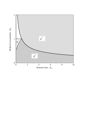
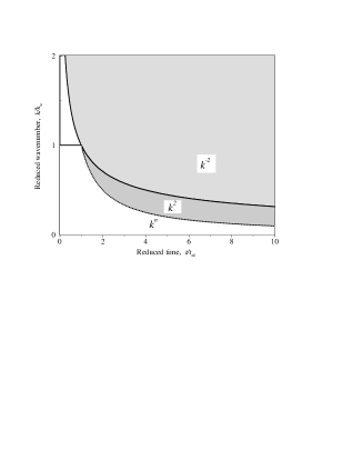
   (a)               (b)

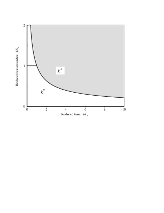
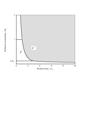
   (c)               (d)

Figure 1: The universal behavior $E(k,t)\sim|k|^{n},k^{2},k^{-2}$ and self-similarity $E(k,t)=L^{3}(t)t^{-2}\tilde{E}(kL(t))$ of the energy spectrum on the $(k-t)$ plane. The line $k_{L}(t)\sim 1/L(t)$ is the border between $k^{-2}$ and $|k|^{n}$ or $k^{2}$ asymptotics of the spectrum. The line $k_{\rm s}(t)$ is the border between $|k|^{n}$ and $k^{2}$ behavior at smal wavenumber. Fig. 1 a - power index $n>2$ : universal self-similar behavior at $t\gg t_{\rm nl}$. Fig. 1 b power index $1<n<2$ : self-similar behavior only when $t\gg t_{\rm nl}$ and $k\gg k_{\rm s}(t)$. Fig. 1 c power index $-3<n<1$ : self-similar behavior for $t\gg t_{\rm nl}$. Fig. 1 d power index $-3<n<1$ and an infrared cutoff $k_{\rm i}$ : self-similar behavior for $t_{\rm i}\gg t\gg t_{\rm nl}$ and $k_{\rm i}\gg k\gg k_{\rm u}$.

Let us now proceed to explain how Fig. 1 can be motivated. From equation (1) we can derive an equation for the velocity potential $\psi$ and by the Hopf-Cole transformation $\psi=2\nu\ln\theta$ Hopf (1950); Cole (1951), we turn this into a linear diffusion equation for an auxiliary field $\theta$. Convolution of the initial data for $\theta$ with the standard heat kernel gives the the solution of diffusion equation, which in the limit $\nu\rightarrow 0$ may be computed by the method of steepest descent. The velocity potential in the limit $\nu\rightarrow 0$ is then

$$\psi(x,t)=\max_{a}\left[\psi_{0}(a)-\frac{(x-a)^{2}}{2t}\right].$$ (2)

where $\psi_{0}(a)$ is the initial potential. The velocity field follows by differentiation in $x$ and reads

$$v(x,t)=-\psi_{x}(x,t)=\frac{x-a(x,t)}{t},$$ (3)

where $a(x,t)$ is the argument of the maximization in (2) for given given $x$ and $t$. If there are several such $a(x,t)$’s, we are at a shock, where the velocity field is discontuous. See e.g.Burgers (1974); Whitham (1974); Gurbatov et al. (1991); Woyczynski (1998) or op. cit. for an in-depth discussion.

In this paper we look at initial conditions with energy spectrum

$$E_{0}(k)=\alpha^{2}|k|^{n}b_{0}(k),$$ (4)

where $n$ is the spectral exponent and $b_{0}(k)$ satisfies $b_{0}(k)=1$ in some regions of wavenumbers [$k_{\rm i},k_{\rm u}$], while going quickly to zero on either side. The (mean) energy is

$$E(t)\equiv\langle v^{2}(x,t)\rangle=\int_{-\infty}^{\infty}E(k,t)\,dk.$$ (5)

and the initial energy is denoted

$$\sigma_{v}^{2}\equiv\langle v_{0}^{2}(x)\rangle=\int_{-\infty}^{\infty}E_{0}(k)\,dk.$$ (6)

It is clear from formula (2) above that the solutions depend solely from the initial velocity potential. Let us introduce the variance of the initial potential (if it exists) :

$$\sigma_{\psi}^{2}\equiv\langle\psi_{0}^{2}(x)\rangle=\int_{-\infty}^{\infty}{E_{0}(k)\over k^{2}}\,dk.$$ (7)

It is also clear that for a continuous initial velocity field the time of first shock formation depends on the initial velocity gradients as $t_{\rm s,first}=-1/\min\partial_{x}v(x,t_{0})$. Consequently, the variance of the initial velocity gradient (if it exists)

$$\sigma_{q}^{2}\equiv\langle(\partial_{x}v_{0}(x))^{2}\rangle=\int_{-\infty}^{\infty}k^{2}E_{0}(k)\,dk.$$ (8)

should also be of interest as it determines the typical time of first shock formation $t_{\rm s}=1/\sigma_{q}$. Since the initial conditions are scaling only in a finite range, all three characteristic quantities $\sigma_{q}$, $\sigma_{v}$ and $\sigma_{\psi}$ exist and are finite. This situation we have always in numerical experiments when $k_{\rm i}$ is determined by the size of box $L_{\rm box}$ and $k_{\rm u}$ is the inverse of the step of discretization. However, depending on $n$, they are dominated by one or the other of the the cutoffs. This suggests hence the following first division of spectral exponents $n$ (see Table 1).

$n$	-3			-1		1
$\sigma_{q}$		$k_{\rm i}$		$k_{\rm u}$		$k_{\rm u}$		$k_{\rm u}$
$\sigma_{v}$		$k_{\rm i}$		$k_{\rm i}$		$k_{\rm u}$		$k_{\rm u}$
$\sigma_{\psi}$		$k_{\rm i}$		$k_{\rm i}$		$k_{\rm i}$		$k_{\rm u}$

Table 1: Division of domains of spectral exponent $n$ according to second moments of $\partial_{x}v_{0}$, $v_{0}$ and $\psi_{0}$. An entry $k_{\rm i}$ and $k_{\rm u}$ indicates that the corresponding quantity is dominated respectively by the low-$k$ and high-$k$ cutoffs.

From the maximum representation of the solutions to Burgers equation (2), we can introduce the scale $L(t)$, proportional to the typical value of $|(x-\tilde{a}(x,t)|$. For large time, balancing the two terms in (2), we have the following prediction for the scale $L(t)$ of Burgers turbulence (see Table 2).

$n$			-3		-1		1
$L(t)$		$(\sigma_{\psi}t)^{1/2}$		$(\alpha t)^{2/(3+n)}$		$(\alpha t)^{2/(3+n)}$		$(\sigma_{\psi}t)^{1/2}$
$E(t)$		$(\sigma_{\psi}t)^{-1}$		$\alpha^{2}k_{\rm i}^{n+1}$		$(\alpha t)^{2(n+1)/(3+n)}$		$(\sigma_{\psi}t)^{-1}$

Table 2: Division of domains of spectral exponent $n$ according to predicted typical scale and energy of solutions to Burgers equation as depending on time $t$.

Here we take into account that the increments of the potential in (2) is $(\psi_{0}(x)-\psi_{0}(0))\sim\alpha x^{(1-n)/2}$ for $n<1$ and is $\sim\sigma_{\psi}$ for $n>1$ Gurbatov et al. (1991); Vergassola et al. (1994). We assume further that $k_{\rm i}=0$ for $n<1$ and that there is some cutoff number $k_{\rm u}$ for $n>1$. In the range $n<-3$ we also need to have $k_{\rm i}>0$ as the solution of Burgers equation exists only if the potential grows slower than quadratically (see the maximum representation (2)) and this implies that the spectrum must be shallower than $k^{-3}$ when $k\to 0$. From the equation (3), we have that at large time between the shocks $x_{{\rm shock},m}<x<x_{{\rm shock},m+1}$ the velocity field has an universal structure $v(x,t)=(x-a_{m})/t$ and so the energy of Burgers turbulence my be estimated as $E(t)\sim L^{2}(t)/t^{2}$ (see Table 2). For the energy to be finite in the range $-3<n<-1$, we require that there is some cutoff wavenumber $k_{\rm i}>0$. It has been known for some time that the behaviour of $L(t)$ and $E(t)$ in $1<n$ has logarithmic corrections Kida (1979); Gurbatov and Saichev (1981); Fournier and Frisch (1983); Gurbatov et al. (1997).

If indeed Burgers turbulence is characterized by a single scale $L(t)$, by dimensional analysis the spectrum takes the following self-similar form:

$$E(k,t)=\frac{L^{3}(t)}{t^{2}}\tilde{E}(kL(t)),$$ (9)

It is well known that for an initial spectrum with $n>2$ the parametric pumping of energy to the area at small $k$’s leads to the universal quadratic law, $E(k,t)\sim k^{2}$, and for $n<2$ we have conservation of initial spectrum $E(k,t)=E_{0}(k)=\alpha^{2}|k|^{n}$ at small wavenumber, which is the spectral form of principle of “permanence of large eddies” (PLE) Frisch (1995); Gurbatov et al. (1997). In Fourier space the self-similarity ansatz (9), together with the PLE gives the same relations for integral scale and the energy as written above, but now in the region $-3<n<2$. Clearly, this argument cannot be applied with initial data such that the spectral index $n\geq 2$, since the later spectrum has now a $k^{2}$ dependence at small $k$ with a time-dependent coefficient. But comparing this with Table 2, where the validity of $L(t)\sim(\alpha t)^{2/(3+n)}$ is $n<1$, we see that the region $1<n<2$ has to be a case apart. In the interval $1<n<2$ the self-similarity ansatz is not correct, as was shown in Gurbatov et al. (1997). The reason for this is competition between the initial $|k|^{n}$ (with constant prefactor $\alpha^{2}$), and the autonomously generated $k^{2}$ (with prefactor increasing in time). If $n>2$, the initial spectrum, at low $k$, is soon overwhelmed by $k^{2}$ generated by nonlinear interactions between harmonics. In this case, hence, the spectrum is fully universal, characterized by a single scale $L(t)$, and otherwise independent of spectral index $n$.

For sufficiently large wave numbers, the spectrum should always be dominated by shocks. In one range, we should therefore have

$$E(k,t)\sim\frac{B(t)}{k^{2}}\qquad\qquad\hbox{$k$ large}$$ (10)

which is equivalent to (9) if $B(t)\sim L(t)/t^{2}$. The amplitude of the small scale part of the spectrum will decrease with time for $n>-2$ and increase with time for $-3<n<-2$.

We note that the spectrum gives only partial information on the solutions to Burgers equation. Indeed, a $k^{-2}$ tail does not distinguish between discontinuous solutions with shocks, and standard Brownian motion, which is almost surely continuous. See She et al. (1992); Sinai (1992); Vergassola et al. (1994) for other characteristics of the mass and velocity distribution.

The rest of the paper will establish the regions in $k$ and $t$ for which the above tables is true if we have cutoff at large and small wave-numbers.

III Homogeneous velocity and homogeneous potential; $(n>1)$ and $(n<-3)$

.

In this chapter we consider the evolution of Burgers turbulence in the region $n>1$ assuming that both velocity and potential are homogeneous Gaussian random function. It means that we necessarily have some ultraviolet cutoff wavenumber $k_{\rm u}$. The function $b_{0}(k)$ can be characterized by a wavenumber $k_{\rm u}$ around which lies most of the initial energy and which is, in order of magnitude, the inverse of the initial integral scale $L_{0}$. Similar situation we have for the spectrum $n<-3$ and cutoff $k_{\rm i}$ at small wave number.

Most of the results about the energy decay for this region have already been obtained by Kida Kida (1979), but for the discrete model of initial condition. He introduced a model of discrete independent potential values in adjacent cells, while their relation to the properties of the initial conditions (say, the spectrum) were left unspecified. For the case of a p.d.f. with a Gaussian tail, he obtained the functional form for the correlation function, energy spectrum and the log-corrected $1/t$ law for the energy decay $E(t)\sim t^{-1}\sigma_{\psi}\ln^{-1/2}\left(t/t_{\rm nl}\right)$, where however in the definition of the nonlinear time $t_{\rm nl}$ was some free parameter - the length of cell in the discrete model. In the more recent contributions Gurbatov and Saichev (1981),Fournier and Frisch (1983) (see also Gurbatov et al. (1991)) the authors conjectured the asymptotic existence of a Poisson process. This was then proved in Molchanov et al. (1995), showing that, in the $x$-$\psi$ plane, the density of the points is uniform in the $x$-direction and exponential in the $\psi$-direction. This permits the calculation of the one- and two-point p.d.f.’s of the velocity Gurbatov and Saichev (1981) and also the full $N$-point multiple time distributions (Molchanov et al. (1995). In papers Gurbatov and Saichev (1981),Fournier and Frisch (1983) was also shown that the statistical properties of the points of contact between the parabola and the initial potential can be obtained from the statistical properties of their intersections, whose mean number can be calculated using the formula of Rice Leadbetter et al. (1983). Thus, it is possible to express the parameters in the asymptotic formulas in terms of the r.m.s. initial potential and velocity.

In the limit of vanishing viscosity, as the time $t$ tends to infinity, the statistical solution becomes self-similar and the energy spectrum has the form (9). The integral scale $L(t)$ and the energy $E(t)$ are given, to leading order, by

$$L(t) \simeq (t\sigma_{\psi})^{1/2}\ln^{-1/4}\left({t\over 2\pi t_{\rm nl}}\right)\ ,$$ (11)

$$E(t) \simeq t^{-1}\sigma_{\psi}\ln^{-1/2}\left({t\over 2\pi t_{\rm nl}}\right)\ ,$$ (12)

where

$$t_{\rm nl}\equiv L_{0}^{2}/\sigma_{\psi}=L_{0}/\sigma_{v},\qquad L_{0}\equiv\sigma_{\psi}/\sigma_{v},$$ (13)

are the nonlinear time and the initial integral scale of turbulence. Using this definition we can rewrite in a first approximation

$$L(t)\simeq L_{0}(t/t_{\rm nl})^{1/2},\qquad E(t)\simeq E_{0}(t/t_{\rm nl})^{-1}.\\$$ (14)

The non-dimensionalized self-similar correlation function $\tilde{B}_{v}(\tilde{x})$, which is a function of $\tilde{x}=x/L(t)$, is given by

$$\tilde{B}_{v}(\tilde{x})={d\over d\tilde{x}}\left(\tilde{x}P(\tilde{x})\right),$$ (15)

where for $x\geq 0$

$$P(\tilde{x})={1\over 2}\int_{-\infty}^{\infty}{dz\over g\left({\tilde{x}+z\over 2}\right)\exp\left[{(\tilde{x}+z)^{2}\over 8}\right]+g\left({\tilde{x}-z\over 2}\right)\exp\left[{(\tilde{x}-z)^{2}\over 8}\right]},$$ (16)

$$g(z)\equiv\int_{-\infty}^{z}e^{-s^{2}/2}\,ds.$$ (17)

Our choice of normalization of the energy as $E(t)=L^{2}(t)/t^{2}$ imposes that for the dimensionless spectrum we have $\int\tilde{E}(\tilde{k})\,d\tilde{k}=1$. It may be shown that the function $P(\tilde{x})$ is the probability of having no shock within an Eulerian interval of length $\tilde{x}L(t)$ Gurbatov et al. (1991).

Note that the properties of the self-similar state are universal in so far as they are expressed solely in terms of two integral characteristics of the initial spectrum, namely the initial r.m.s. potential $\sigma_{\psi}$ and r.m.s. velocity $\sigma_{v}$. Observe that the spectral exponent does not directly enter, in contrast to what happens when $n<1$ (see sections IV,V). For the dimensionless spectrum

$$\tilde{E}(\tilde{k}) = \frac{1}{2\pi}\int_{-\infty}^{\infty}\tilde{B}_{v}(\tilde{x})\exp(i\tilde{k}\tilde{x})\,d\tilde{x}$$ (18)

$$= -\frac{ik}{2\pi}\int_{-\infty}^{\infty}\tilde{x}P(\tilde{x})\exp(i\tilde{k}\tilde{x})\,d\tilde{x},$$

we have the following asymptotic:

$$\tilde{E}(\tilde{k})\simeq\left\{\begin{array}[]{rl}a_{+}\,{\tilde{k}}^{2},&\tilde{k}\ll 1\\[6.45831pt] a_{-}\,{\tilde{k}}^{-2},&\tilde{k}\gg 1\\ \end{array}\right.,\quad\tilde{k}\equiv kL(t)\ .$$ (19)

The $k^{-2}$ region is the signature of shocks, while the $k^{2}$ region comes due to the parametric pumping of energy to the area of small $k$. The two constants $a_{+}$ and $a_{-}$ can be computed theoretically as Gurbatov et al. (1991)

$$a_{+} = 1/\pi\int_{0}^{\infty}\tilde{x}^{2}P(\tilde{x})\,d\tilde{x}=1.078\ldots$$

$$a_{-} = 2\pi^{-3/2}=0.359\ldots$$ (20)

In dimensioned variables, the small-$k$ region behavior of the spectrum is thus

$$E(k,t)=a_{+}\frac{L^{5}(t)}{t^{2}}\,k^{2}=A(t)\,k^{2},\quad kL(t)\ll 1,$$ (21)

where

$$A(t)\simeq a_{+}\sigma_{v}^{2}L_{0}^{3}\left(\frac{t}{t_{\rm nl}}\right)^{\frac{1}{2}}\,\ln^{-5/4}\left(\frac{t}{2\pi t_{\rm nl}}\right).$$ (22)

So, we have a spectrum with an algebraic $k^{2}$ region and a time-increasing coefficient $A(t)$.

The situation is more complicated at large but finite time Gurbatov et al. (1997). We must now distinguish two cases. When $n>2$, the $k^{2}$ contribution (21) dominates everywhere over the $|k|^{n}$ contribution and we have a self-similar evolution in the whole range of wavenumbers (see Fig. 1 a), but the “self-similar” time $t_{\rm ss}$ from which we have self-similar stage of evolution depends on $n$. In the general case, the condition $t/t_{\rm nl}\gg 1$ is not enough for the Poisson approximation to hold and consequently for the existence of self-similarity. Let us denote by $\Delta_{\rm corr}$ a typical correlation length for the initial potential, which may be greater the initial integral scale $L_{0}$. The self-similarity occurs when the integral scale of the turbulence $L(t)$ (11) is much greater the typical correlation length $\Delta_{\rm corr}$. This leads to the following condition on the “self-similar” time $t_{\rm ss}$ Gurbatov et al. (1997)

$$t_{\rm ss}\sim t_{\rm nl}\left(\frac{\Delta_{\rm corr}}{L_{0}}\right)^{2}\ .$$ (23)

There are instances where $(\Delta_{\rm corr}/L_{0})^{2}$ can be large. Consider an initial spectrum $E_{0}(k)$ (4) with $n\gg 1$ and a function $b_{0}(k)$ decreasing rather fast when $k>k_{\rm u}$. In this case the initial velocity field is a quasi-monochromatic signal with a center wavenumber $k_{\rm u}\sim L_{0}^{-1}$ and a width $\Delta k\sim\left[\Delta_{\rm corr}\right]^{-1}\ll k_{\rm u}$. At the early stage of evolution $t_{\rm nl}\ll t\ll t_{\rm nl}(\Delta_{\rm corr}/L_{0})$ we have the saturation of amplitude modulation and the shift of the shocks is much smaller then the period of the quasi-monochromatic signal. The energy of this signal is approximately the same as the energy of the periodic wave : $E(t)\simeq L_{0}^{2}/12t^{2}$ Gurbatov and Malakhov (1977). Nevertheless due to the finite width of the initial spectrum, we have the generation of a low frequency component $v_{l}(x,t)$ whose spectrum is well separated from the primary harmonic $k_{\rm u}$ and with the energy $E_{l}(t)\sim E_{0}(L_{0}/\Delta_{\rm corr})^{2}\ll E_{0}$. At $t_{\rm nl}(\Delta_{\rm corr}/L_{0})\ll t\ll t_{\rm nl}(\Delta_{\rm corr}/L_{0})^{2}$ the energy of the low frequency component is larger than the energy of the high-frequency quasi-periodic wave, but to the large spatial scale we have a relatively small distortion of this component. And only at $t\gg t_{\rm ss}\sim t_{\rm nl}(\Delta_{\rm corr}/L_{0})^{2}$ do we have the self-similar regime of evolution. The physical reason for this is a strong correlation of the shocks in the early stage of the evolution, which prevents the rapid merging of shocks. We need to stress that we have a similar situation for a spectrum $n\ll-3$ and a cutoff $k_{\rm i}$ at small wave number.

Figure 2: Evolution of the energy spectrum with an initial spectrum proportional to $k^{4}$ at small wavenumbers $k$. The spatial resolution is $N=2^{20}$. Spectra averaged over 3000 realizations. The labels correspond to output times $t/t_{\rm nl}=0.033$,…, up to $t/t_{\rm nl}=3.3\times 10^{8}$.

Figure 3: Reduced energy spectra $E(k,t)t^{2}/L_{\rm exp}^{3}(t)$ ($n=4$) at the same times as a function of reduced wave number $kL_{\rm exp}(t)$.

Let us now discuss the results of numerical simulations. We use a smooth cutoff of the initial power spectrum (43) with $k_{\rm u}=N/16$. We consider in all experiments periodic initial condition, so the infra-red cutoff frequency in this case is determined by the size of simulation box and $k_{\rm i}=2\pi$. To check the self-similar ansatz we consider the evolution of energy spectrum $E(k,t)$, of the energy $E(t)=\langle v^{2}(x,t)\rangle$ and of the integral scale $L_{\rm exp}(t)$ which we can measure from the experimental data as

$$L^{2}_{\rm exp}(t)=\langle\psi^{2}(x,t)\rangle/\langle v^{2}(x,t)\rangle\ .$$ (24)

In Fig. 2 energy spectra (averaged over about $3000$ realizations of the random process) are shown at different moments of time from $t/t_{\rm nl}=0.033$ to $t/t_{\rm nl}=3.3\times 10^{8}$. The initial spectrum was $k^{4}$ at small $k$. Fig. 3 contains reduced energy spectra $E(k,t)t^{2}/L_{\rm exp}^{3}(t)$ at the same time as a function of reduced wave number $kL_{\rm exp}(t)$. We see the generation of $A(t)\,k^{2}$ with growing amplitude $A(t)$ at small $k$, and $k^{-2}$ at large wavenumber. The switch point $k_{\rm s}(t)$ between $A(t)k^{2}$ and $\alpha^{2}|k|^{n}$ regions of the spectrum moves quickly towards the maximum of the spectrum and finally the $\alpha^{2}k^{4}$ part of the spectrum disappears (see Fig. 1a).

The preservation of the shape of each curve at large time $t/t_{\rm nl}>10$ is evident. It is also seen that the total energy (the area under the curves) decreases, and so does the characteristic wavenumber $k_{L}(t)\sim 1/L(t)$. The curves in Fig. 3 have been plotted with respect to the reduced wavenumber $k\,L_{\rm exp}(t)$ as the quantity $L_{\rm exp}(t)$ can be measured unambiguously from the numerical simulations. To compare the results with the spectrum theoretical $\tilde{E}(\tilde{k})$ (18), we need to deduce the relation between $L_{\rm exp}(t)$ and $L(t)$, that we can get from (9)

$$L^{2}_{\rm exp}(t) = L^{2}(t)\frac{\int_{-\infty}^{\infty}\tilde{E}(\tilde{k})\tilde{k}^{-2}\,d\tilde{k}}{\int_{-\infty}^{\infty}\tilde{E}(\tilde{k})\,d\tilde{k}}$$ (25)

$$= L^{2}(t)\int_{0}^{\infty}\tilde{x}P(\tilde{x})\,d\tilde{x}\approx 1.65\ L^{2}(t).$$

From these, we deduce the experimental values of the constants $a_{+}=1.10$ and $a_{-}=0.37$, both slightly larger ($\approx$ 2 %) than the theoretical values. This very small discrepancy could be due to finite-size effects contaminating the measurement of $\langle\psi^{2}(x,t)\rangle$ at small wavenumbers and $\langle v^{2}(x,t)\rangle$ at large wavenumbers, and thus of the experimental integral scale $L_{\rm exp}(t)$.

The asymptotic spectrum is reached rather quickly after the non-linear time $t_{\rm nl}$ and the asymptotic formula describes the numerical data very well, not only in the limits of relatively large and small wave numbers, but also at the top, where the spectrum switches between the two asymptotes. From Fig. 3 is also seen that the transition between the two asymptotics $\tilde{k}^{2}$ and $\tilde{k}^{-2}$ is rather sharp.

III.1 Breakdown of self-similarity; $(1<n<2)$

The more interesting case is $1<n<2$, when we have breakdown of the self-similarity Gurbatov et al. (1997). The permanence of large eddies implies now that, at extremely small $k$,

$$E(k,t)\simeq\alpha^{2}|k|^{n},\quad{\rm for}\,\,k\to 0.$$ (26)

This relation holds only in an outer region $|k|\ll k_{\rm s}(t)$ where (26) dominates over (21). The switching wavenumber $k_{\rm s}(t)$, obtained by equating (21) and (26), is given by

$$k_{\rm s}(t) \simeq \left(\frac{\alpha^{2}t^{2}}{L^{5}(t)}\right)^{\frac{1}{2-n}}$$ (27)

$$\simeq L_{0}^{-1}\left(\frac{t}{t_{\rm nl}}\right)^{-\frac{1}{2(2-n)}}\ln^{\frac{5}{4(2-n)}}\left(\frac{t}{2\pi t_{\rm nl}}\right).$$

Let us define an energy wavenumber $k_{L}(t)=L^{-1}(t)$, which is roughly the wavenumber around which most of the kinetic energy resides. From (11) $k_{L}(t)\sim(t\sigma_{\psi})^{-1/2}$ (ignoring logarithmic corrections). We then have from (27), still ignoring logarithmic corrections :

$$\frac{k_{\rm s}(t)}{k_{L}(t)}\sim\left(\frac{t}{t_{\rm nl}}\right)^{-\frac{n-1}{2(2-n)}}.$$ (28)

Hence, the switching wavenumber goes to zero much faster than the energy wavenumber, so that the preserved part of the initial spectrum $|k|^{n}$ becomes rapidly irrelevant. Let us also observe that the ratio of the energy in the outer region to the total energy, a measure of how well the Kida law (11) is satisfied, is equal to $(t/t_{\rm nl})^{-3(n-1))/(n-2)}$ (up to logarithms) and thus becomes very small when $t\gg t_{\rm nl}$, unless $n$ is very close to unity. Thus, for $1<n<2$ there is no globally self-similar evolution of the energy spectrum at finite time. Of course, as $n\to 2$ the inner $k^{2}$ region overwhelms the outer $|k|^{n}$ region and as $n\to 1$ the converse happens, so that in both instances global self-similarity tends to be reestablished.

Figure 4: Evolution of the energy spectrum with an initial spectrum proportional to $|k|^{n}$ ($n=1.5$) at small wavenumbers $k$. Resolution $N=2^{20}$. The labels correspond to output times $t_{1}/t_{\rm nl}=0.18$,…, up to $t/t_{\rm nl}=1.8\times 10^{10}$.

Figure 5: Reduced energy spectra $E(k,t)t^{2}/L^{3}(t)$ at the same times as a function of reduced wave number $kL(t)$ using the theoretical value $L(t)=(t/t_{\rm nl})^{1/2}[\log(t/2\pi t_{\rm nl})]^{-1/4}$.

In Fig. 4 energy spectra (averaged over $\sim 3000$ realizations of the random process) are shown at different moments of time from $t/t_{\rm nl}=0.18$ to $t/t_{\rm nl}=1.8\times 10^{10}$. For the initial spectrum we have $n=1.5$. Fig.  5 contains reduced energy spectra $E(k,t)t^{2}/L^{3}(t)$ at the same time as a function of reduced wave number $kL(t)$, when we use the asymptotic expression (11) for $L(t)$. We see again the generation of $A(t)\,k^{2}$ with growing amplitude $A(t)$ at small $k$ and $k^{-2}$ at large wavenumber. The switch point $k_{\rm s}(t)$ between $A(t)\,k^{2}$ and $\alpha^{2}|k|^{n}$ regions of the spectrum tends slowly to the origin of the spectrum and finally the $\alpha^{2}|k|^{n}$ part of the spectrum disappears (see Fig. 1 b).

Figure 6: Evolution of the computed integral scale $L_{\rm exp}(t)$ for $n=1.5,2,3,4$ (dotted lines) compared to the theoretical leading-order prediction $\tilde{L}_{\rm exp}=1.28\,L(t)$ (11),(25) (solid line) and the same without the logarithmic correction (dashed line).

Figure 7: Evolution of the computed integral energy $E(t)$ for $n=1.5,2,3,4$ (dotted lines) compared to the theoretical leading-order prediction $E(t)=L^{2}(t)/t^{2}$ (12) (solid line) and the same without the logarithmic correction (dashed line).

Thus the numerical experiments support the theoretical prediction that for $n>1$ at large time we have the self-similar behavior of the spectrum (9). Moreover the integral scale of turbulence $L(t)$(11) and the energy of turbulence $E(t)$ are in perfect agreement with theoretical predictions, even for $1<n<2$ where we have breaking of self-similarity. On Fig. 6 and 7 we plot the evolution of $L_{\rm exp}(t)$ and $E(t)$ for different $n=1.5,2,3,4$ and the theoretical curves, taking into account the relation between $L_{\rm exp}(t)$ and $L(t)$ (25), showing that the theoretical predictions are perfectly reproduced by the simulations.

In all experiments, we only consider times small enough for the characteristic wavenumber $k_{L}(t)\gg k_{\rm i}$, so that we still have many shocks in the box. When this condition is broken, it means we have a single shock in the simulation domain and we have universal self-similar linear decay of the spectrum $E(k,t)\sim(kt)^{-2}$.

IV Homogeneous velocity and non-homogeneous potential; $(-1<n<1)$

We begin with the case $-1<n<1$ when the initial potential has homogeneous increments. Many aspects of this case are well understood, thanks in particular to Burgers’ own work Burgers (1974), who did consider the case when the initial velocity is white noise $n=0$ (see also Gurbatov et al. (1991); Woyczynski (1998)).

The phenomenology is quite simple (see section II). Increments $\Delta\psi_{0}(L((t))$ of the initial potential over a distance $L(t)=x-\tilde{a}(x,t)$ can be estimated from the square root of the structure function $S_{0\psi}(L)$ of the potential (29)

$$S_{0\psi}(x)\equiv\langle\left(\psi_{0}(x)-\psi_{0}(0)\right)^{2}\rangle,$$ (29)

When when $n<1$, it grows without bound $S_{0\psi}(x)\sim\alpha^{2}|x|^{1-n}$. For a given position $x$, the maximum in (2) will come from those $a$s such that the change in potential is comparable to the change in the parabolic term and this immediately leads to $L(t)\sim\alpha t^{2/(n+3)}$. (see Table (2).

When the initial spectrum (4) has no cutoff wavenumber, we can use that scaling and then get immediately that the above mentioned expression for the integral scale $L(t)$ and energy $E(t)$ (see Table 2) are now exact for all time starting from zero. For details, see Vergassola et al. (1994) (Section 4) and Avellaneda and E (1995). But even when the initial spectrum has both cutoff waves numbers at large and small scale there is some region in ($kt$) plane where we have self-similar evolution of the spectrum.

In the general case for the structure function (29) of the potential, we have

$$S_{0\psi}(x) = g(x)\beta^{2}\alpha^{2}|x|^{1-n}\ ,$$

$$\beta^{2} = \alpha^{2}{{2\pi}\over{\Gamma(2-n)\sin\frac{\pi(n-1)}{2}}}$$ (30)

The properties of the dimensionless function $g(x)$ are determined by the function $b(k)$ and for $b(k)\equiv 1$ we have $g(x)\equiv 1$. When the initial spectrum has cutoff wavenumbers $k_{\rm i}$ and $k_{\rm u}$ the function $g(x)=1$ in some spatial interval $L_{\rm u}<x<L_{\rm i}$ where $L_{\rm u}\sim 1/k_{\rm u}$ and $L_{\rm i}\sim 1/k_{\rm i}$. Let us introduce the dimensionless variables

$$\tilde{x}=x/L(t),\qquad\tilde{a}=a/L(t),\qquad\tilde{v}=v/(L(t)/t),$$ (31)

where $L(t)$ is an integral scale of turbulence. Then the “maximum representation” will be rewritten in the form

$$\tilde{v}(\tilde{x},t)=\tilde{x}-\tilde{a}(\tilde{x},t),$$ (32)

where $\tilde{a}(\tilde{x},t)$ is the coordinate at which dimensionless function $\tilde{\Phi}(\tilde{x},\tilde{a},t)$ achieves its (global) maximum for given $\tilde{x}$ and $t$ and

$$\tilde{\Phi}(\tilde{x},\tilde{a},t)=\tilde{\psi}_{0}(\tilde{a},t)-\frac{(\tilde{x}-\tilde{a})^{2}}{2}.$$ (33)

here $\tilde{\psi}_{0}(\tilde{a},t)=\psi_{0}(\tilde{a}L(t))\left(t/L^{2}(t)\right)$ is the dimensionless initial potential with the following structure function

$$\tilde{S}_{0\psi}(\tilde{x})=g(\tilde{x}L(t))\beta^{2}|\tilde{x}|^{1-n}$$ (34)

Here we define that integral scale $L(t)$ by the relation

$$L(t)=(\alpha t)^{2/(3+n)}$$ (35)

and so in (34) we use that $(\alpha t)^{2}/L^{(3+n)}(t)=1$. For this definition of the integral scale, we have for the dimensionless spectrum (9)

$$\tilde{E}(\tilde{k})=\left\{\begin{array}[]{rl}{\tilde{k}}^{n},&\tilde{k}\ll 1\\[6.45831pt] \gamma_{n}{\tilde{k}}^{-2},&\tilde{k}\gg 1\\ \end{array}\right.,\quad\tilde{k}\equiv kL(t).$$ (36)

and for the energy of Burgers turbulence

$$E(t)=a_{n}L^{2}(t)/t^{2}=a_{n}\alpha^{\frac{4}{3+n}}t^{-\frac{2(n+1)}{3+n}}$$ (37)

where $\gamma_{n}$ and $a_{n}$ are dimensionless constants, which we will determine from the numerical experiments.

Consider first the case when we have a cutoff wavenumber $k_{\rm u}$ only at small scale ($k_{\rm i}=0$). For $L(t)\gg L_{\rm u}$ the structure function (35) my be replaced by

$$\tilde{S}_{0\psi}(\tilde{x})=\beta^{2}|\tilde{x}|^{1-n},$$ (38)

the function not depending on time and possessing no spatial scales in its own. In this case the statistical properties of absolute maxima coordinates $\tilde{a}$ do not vary with time. The latter phenomenon means that the field $\tilde{v}(\tilde{x},t)$ (32) statistical properties determined by time-independent statistics of $\tilde{a}(\tilde{x},t)$ are rendered self-similar according (32). So at large times when $L(t)$ is also large, we have self-similar evolution of the spectrum Eq.(9) (see Fig. 1 c). Alternatively, we could argue that when $t$ is so large that the parabolas appearing in (2) have a radius of curvature much larger than the typical radius of curvature of features in the initial potential, we can plausibly replace that initial potential by fractional Brownian motion of exponent $h=(1-n)/2$, so that the upper cutoff $k_{\rm u}$ becomes irrelevant. Without loss of generality we may assume that this fractional Brownian motion starts at the origin for $x=0$. This function is then statistically invariant under the transformation $x\to\lambda x$ and $\psi_{0}\to\lambda^{h}\psi_{0}$. It is then elementary, using (2), to prove that a rescaling of the time is (statistically) equivalent to a suitable rescaling of $x$ distances and of $\psi(x,t)$. This implies the above expression for $L(t)$ and $E(t)$ (see Table 2).

For the self-similar initial spectrum with $-1<n<1$ we have a divergence of the potential in the infrared part of the spectrum and divergence of velocity and gradient at small scale. So we can not introduce now the initial scale on the base of (13). Assuming that we have a cutoff wavenumber at small scale, we can in this section use some other definition of nonlinear time and initial scale

$$t^{{}^{\prime}}_{\rm nl}=L^{{}^{\prime}}_{0}/\sigma_{v}=1/\sigma_{q},\qquad L^{{}^{\prime}}_{0}\equiv\sigma_{v}/\sigma_{q},$$ (39)

It is easy to see that this time is equal to the the characteristic time of shock formation $t_{\rm s}$. Using this definition we can rewrite the expression for $L(t)$ and $E(t)$ in the form

$$L(t) \simeq L^{{}^{\prime}}_{0}(t/t^{{}^{\prime}}_{\rm nl})^{2/(3+n)},$$ (40)

$$E(t) \simeq E_{0}(t/t^{{}^{\prime}}_{\rm nl})^{-2(n+1)/(3+n)}.$$ (41)

Assume now that we have also a cutoff wavenumber $k_{\rm i}$ at large scale and we have saturation of the potential structure function to $2\sigma^{2}_{\psi}$ at $x\gg L_{\rm i}$. In this case in the interval when $L_{\rm i}\gg L(t)\gg L_{\rm u}$ we can replace the dimensionless structure function (35) by (38). It means that in some time interval $t_{\rm u}\ll t\ll t_{\rm i}$, where $t_{\rm u}$, $t_{\rm i}$ are determined by the condition $L(t_{\rm i})=L_{\rm i}$, $L(t_{\rm u})=L_{\rm u}$, we will still have self-similar laws for the integral scale $L(t)$ and energy $E(t)$ of turbulence. The energy spectrum $E(k,t)$ will have the self-similar behavior on this time in the region $k>k_{\rm i}$ (see Fig. 1 d). For the final state at very large times, there are two possible situations. In the first one, if we have a finite box of size $L_{\rm box}=L_{\rm i}=2\pi/k_{\rm i}$ and a periodic initial perturbation with this period, then at very large time we will finally have one triangular wave on the period and the energy will be decay as $E(t)=L^{2}_{\rm i}/12t^{2}$. In the non-periodic case with a continuous power spectrum, we will have the generation of a low frequency component $E(k,t)\sim A(t)\,k^{2}$ in region $k<k_{\rm i}$ and finally the behavior of the turbulence will be like in the case $n>1$ (see section III).

In numerical simulations we used two models of initial spectrum. In the first one we assume that we have the self-similar power spectrum (4) in the whole wavenumber range from $2\pi$ to $N\pi$ ($k_{\rm i}=2\pi$, $k_{\rm u}=N\pi$), in the second we use an infrared cutoff wavenumber $2\pi\ll k_{\rm i}\ll k_{\rm u}=N\pi$. If the initial spectrum is self-similar inside the interval $k_{\rm i}=2\pi$,$k_{\rm u}=N\pi$ then for the nonlinear time $t^{{}^{\prime}}_{\rm nl}$ we have

$$t^{{}^{\prime}}_{\rm nl} = \left(\frac{n+3}{2}\right)^{1/2}\frac{1}{\alpha(k_{\rm u}^{(3+n)/2}-k_{\rm i}^{(3+n)/2})}$$ (42)

$$\simeq \left(\frac{n+3}{2}\right)^{1/2}\frac{1}{\alpha k_{\rm u}^{(3+n)/2}}\ .$$

Figure 8: Evolution of the energy spectrum with an initial spectrum proportional to $|k|^{n}$ ($n=0.5$) at small wavenumbers $k$. Resolutions $N=2^{15}$ and $N^{\prime}=2^{20}$ are denoted by filled or open symbols respectively. The labels correspond to output times $t_{1}=1.5\cdot 10^{-7}$,…, up to $t=1.5\cdot 10^{-3}$ (in absolute time, the reduced time $t/t^{{}^{\prime}}_{\rm nl}$ depends on the value of the upper cutoff $k_{\rm u}$, equal in this case to $N\pi$ or $N^{\prime}\pi$).

Figure 9: Reduced energy spectra $E(k,t)\,t^{2/7}$ ($n=0.5$) at the same times as a function of reduced wave number $k\,t^{4/7}$. Same conditions as in Fig. 8.

In Fig. 8 energy spectra $E(k,t)$ are shown at different moments of time from $t/t^{{}^{\prime}}_{\rm nl}=21$ to $t/t^{{}^{\prime}}_{\rm nl}=9.1\times 10^{7}$. The initial spectrum was $|k|^{n}$ with $n=0.5$, but two simulations were done with different resolutions $N=2^{15}$ and $N^{\prime}=2^{20}$, so that we have in reality two different ultraviolet cutoffs $k_{\rm u}=2^{15}\pi$ and $k_{\rm u}^{\prime}=2^{20}\pi$. From the figures, one can easily see that in the frequency range $k_{\rm i}<k<\min(k_{\rm u},k_{\rm u}^{\prime})$ the spectra are exactly equal to each other for all times. Fig. 9 shows reduced energy spectra $E(k,t)\,t^{2/7}$ as a function of reduced wave number $k\,t^{4/7}$ at different times for these two different values of $N$. We see that once again, both spectra display a perfectly self-similar evolution and are exactly equal in their common range of reduced wavenumbers. Moreover, it possible to show that we have not only the conservation of the spectrum in presence of high frequency signal but also the conservation of the large-scale structures in each unique realization Aurell et al. (1993); Gurbatov and Pasmanik (1999). The measured value of the dimensionless constant $\gamma_{1/2}=1.62$ is reported in Table 3.

Figure 10: Evolution of the energy spectrum with an initial spectrum independent of $k$ ($n=0$) (white noise initial velocity).

Figure 11: Reduced energy spectra $E(k,t)\,t^{0}$ ($n=0$) at the same times as a function of reduced wave number $k\,t^{2/3}$.

Similarly, in Fig. 10, energy spectra $E(k,t)$ are shown at different moments of time from $t/t^{{}^{\prime}}_{\rm nl}=1.6$ to $t/t^{{}^{\prime}}_{\rm nl}=5.4\times 10^{4}$ for the initial spectrum was a classical white noise with $n=0$. Fig. 11 contains reduced energy spectra $E(k,t)\,t^{0}$ as a function of reduced wave number $k\,t^{2/3}$ at five different time. The observed value of the dimensionless constant $\gamma_{0}=1.43$ is reported in Table 3.

Figure 12: Evolution of the difference of the reduced energy spectrum with the initial white noise spectrum $k^{0}$, showing the universal $k^{2}$ term at small $k$s, which is subleading in this case.

From the structure of the Burgers equation we see that due to nonlinear interaction of harmonics we have always the $k^{2}$ term at low wave numbers $k$, which may be leading or sub-leading. The sign of this term depends on the initial spectrum. It is evident, that for $n>2$ we have generation of new component at small wave number and this term increases with time see equation (22). When $n<2$, this term is subleading, but its growing amplitude can make it apparent so that it dominates the dynamics, as shown in section III.1. But when $n<1$, this term is completely masked by the initial components $\sim|k|^{n}$, and the only way to show that it is really present is by computing the diference of the spectrum with the initial one, provided the statistical noise in the simulations is small enough. This has been done in Fig. 12), showing this subleading term $\sim k^{2}$, this time with a negative amplitude, but displaying also perfect self-similar behavior.

Figure 13: Evolution of the energy spectrum with an initial spectrum independent of $k$ ($n=0$) as a function of reduced wave number $kt^{2/3}$ with an initial infrared cutoff wavenumber at $k_{\rm i}=64\,\pi$ (corresponding to $1/32$ of the box size). One can see that the upper part of the spectrum is unchanged with respect to Fig. 11.

Another way to display this universal low wavenumber $k^{2}$ component, is to introduce some infrared cutoff in the initial condition. In the simulation shown in Fig. 13, we consider the case of white noise initial spectrum $n=0$ but with an infrared cutoff at $k_{\rm i}=64\,\pi$. For the first two displayed times, we have a self-similar evolution of the spectrum in the wave-number range $k_{\rm i}<k<k_{\rm u}$, but with the generation of a component spectrum $E(k,t)\sim A(t)\,k^{2}$ in the region $k<k_{\rm i}$. At the time $t/t^{{}^{\prime}}_{\rm nl}=1.6\cdot 10^{3}$, $L(t)\sim L_{\rm i}$ reaches the lower cutoff $k_{\rm i}$, and the spectrum then becomes equivalent and evolve in time as in section III, where we have self-similar evolution with universal behavior of the spectrum $E(k)\sim k^{2}$ and $E(k)\sim k^{-2}$ at small and large wavenumber respectively. It is interesting to note that all parts of the spectrum $k^{2}$, $k^{0}$ and $k^{-2}$ evolve in a self-similar way for intermediate times $t^{{}^{\prime}}_{\rm nl}<t<t_{\rm i}$.

Figure 14: Evolution of the computed integral energy $E(t)$ for $n=1,0.5,0,-0.5$.

On Fig. 14 the evolution of the energy $E(t)$ for different $n=1,0.5,0,-0.5$ is plotted. The law of decay is in good agreement with the theoretical prediction (41) for all time. The constants $a_{n}$ have been measured and are shown in Table 3.

$n$	-2.5	-2.0	-1.5	-1.0	-0.5	0.0	0.5	1.0
$\gamma_{n}$	$-$	0.94	0.97	1.09	1.26	1.43	1.62	1.93
$a_{n}$	$-$	$-$	$-$	$-$	0.43	0.32	0.32	0.37

Table 3: Measured values of the universal constants $\gamma_{n}$ and $a_{n}$ characterizing the $k^{-2}$ spectrum shock tail and law of energy decay respectively. Values marked $-$ don’t exist or couldn’t be measured.

V Non-homogeneous velocity and non-homogeneous potential potential; $(-3<n<-1)$

For the self-similar initial spectrum with $-3<n<-1$ we have a divergence of the potential and the velocity in the infrared part of the spectrum, and of the gradient in the ultraviolet part. Assuming that we have a cutoff wavenumber at small scale $k_{\rm i}$, we can still use the definition of the nonlinear time through the gradient of velocity $t^{{}^{\prime}}_{\rm nl}=1/\sigma_{q}$ (39), which is equal to the the characteristic time of shock formation $t_{\rm s}$. Due to the divergence of the energy in the infrared part of the spectrum, the dissipation in the shocks doesn’t lead to a finite value of the energy at any time, if there is no cutoff $k_{\rm i}$. Nevertheless we can still introduce the integral scale of turbulence $L(t)$ showing the region when initial power law spectrum $E(k,t)\sim|k|^{n}$ transforms to the universal spectrum $E(k,t)\sim k^{-2}$ . For the spectral form of principle of “permanence of large eddies”, we still have that integral scale grows according (35). From equation (10), we see that the amplitude of small scale part of the spectrum decreases for $n>-2$ and increases with time for $-3<n<-2$.

Figure 15: Evolution of the energy spectrum with an initial spectrum proportional to $k^{-2}$. One can see that the spectrum doesn’t change at all until the non-linear time of the smallest wavenumber component is reached (near $t\approx 0.15$).

Let as start for the special case of initial spectrum with the critical index $n=-2$ when $L(t)\sim(\alpha t)^{2}$. From equation (9), we see that the spectrum does not change in time. In Fig. 15, energy spectra $E(k,t)$ are shown at different moments of time from $t/t^{{}^{\prime}}_{\rm nl}=0.005$ to $t/t^{{}^{\prime}}_{\rm nl}=5$. And we really see that it is only when $t/t^{{}^{\prime}}_{\rm nl}\gg 1$ that the spectrum begins to change, simply decaying in amplitude without changing its shape. But even if it is not apparent in the spectrum, we have an evolution in time of each realization and of other statistical properties, like shock probability distribution or higher moments of the velocity.

Figure 16: Evolution of the velocity field for one particular realization with an initial spectrum $k^{-2}$. Upper plot is the Gaussian Brownian motion initial condition at $t=0$ and lower plot is the velocity field at $t=0.15$, just before the decay of the smallest wavenumber component. Both signals have the same power spectrum. Note that the largest scales are non-linearly distorted, but their amplitude is globally preserved, illustrating the principle of persistence of large eddies.

Figure 17: Reduced energy spectra $E(k,t)\,t^{-4}$ as a function of the reduced wavenumber $k\,L(t)=k\,t^{2}$ for an initial spectrum $k^{-2}$. Note that the spectrum rescaling works even if this case with a factor decreasing with time, and allows the separation of the $k^{-2}$ spectra in differents zones coming from the initial conditions ($k\,L(t)<1$) of from the shocks ($k\,L(t)>1$).

On Fig. 16, the evolution of a realization of a velocity field with a $k^{-2}$ spectrum is plotted at different times. It is easy to see, that even if the spectrum does not change, the characteristic distance between the shocks which is proportional to the scale $L(t)$ increases with time. The signal switches continuously from a Gaussian Brownian motion with random phases to a triangular wave with aligned phases, but these signals have the same power spectrum, and the amplitude of the spectrum is preserved by the Burgers evolution. The evolution of the spectrum in numerical simulations starts and the energy begins to decay at the time $t_{\rm nl,1}$ when the integral scale of turbulence $L(t)$ reaches the size of the box $L_{\rm box}$. This can also be seen in Fig. 17 showing the spectra rescaled with time for Gaussian Brownian motion initial conditions. One can see that the initial $k^{-2}$ spectrum visible for $k\,L(t)<1$ is continuated with the $k^{-2}$ spectrum of the shocks at late times for $k\,L(t)>1$, but that the rescaling allows the separation of both. For a given finite-size realization of the signal with both lower and upper wavenumber cutoffs $k_{\rm i}$ and $k_{\rm u}$, the spectrum will slide along the curve in Fig. 17 until $k_{\rm i}\,L(t)>1$, that is the rescaled wavenumbers $k\,L(t)>1$ are larger than 1 for all $k$s, at which time the spectrum will begin to decay linearly (as shown in Fig. 17 for $t/t^{{}^{\prime}}_{\rm nl}>27$).

Figure 18: Evolution of the energy spectrum with an initial spectrum proportional to $|k|^{-2.5}$. One can see that the amplitude of the high-frequency components increase with time, the $|k|^{-2.5}$ spectrum transforming to a $k^{-2}$ tail, whose energy really comes from the smallest wavenumber components. These have a very slightly decreasing amplitude, so that the global energy is nearly constant, but slightly decays in time.

In fig. 18 the energy spectra $E(k,t)$ with an initial power law spectrum $E(k,t)\sim|k|^{n}$ with $n=-2.5$ is shown at different moments of time from $t/t^{{}^{\prime}}_{\rm nl}=6.9\times 10^{-2}$ to $t/t^{{}^{\prime}}_{\rm nl}=6.9$. We see the generation of universal $k^{-2}$ tail which amplitude increases with time and switching point between $k^{-2.5}$ and $k^{-2}$ parts of the spectrum moved to the small wavenumbers. The value of dimensionless constant $\gamma_{n}$ in the dimensionless spectrum in (36) are shown in Table 3. Note that the constant for $n=-2.5$ has not been measured as the energy begins to decay immediately as soon as the $k^{-2}$ tail is established. This effect also perturbs the measurement of $\gamma_{n}$ for $n<-1$, because in a finite-size system, some (small) dissipation occurs as soon as shocks are present, and so the amplitude of the $k^{-2}$ tail is diminished. This explains why we measure for instance an amplitude $\gamma_{-2}=0.94$ at large times, even if $\gamma_{-2}=1.0$ should be observed.

Figure 19: Evolution of the computed integral energy $E(t)$ for $n=-1.5,-2,0,-2.5$ as a function of $t/t^{{}^{\prime}}_{\rm nl}$.

We can also introduce the other nonlinear time is a time of nonlinear decay of first harmonic $t_{\rm nl,1}=k_{1}/A_{1}$. For $-3<n<1$, we have no significant decay of the energy of turbulence until $t\geq t_{\rm nl,1}$. The constancy of the energy until much later than $t^{{}^{\prime}}_{\rm nl}$ is also evidenced in Fig. 19 for $n=-1.5,-2,-2.5$. As the energy doesn’t decay until $t_{\rm nl,1}$, the “constants” $a_{n}$ don’t exist for $n<-1$ and are thus not shown in Table 3.

VI Discussion

In this work we have reconsidered again the classical problem of the spectral properties of solutions of Burgers’ equation for long times, when the initial velocity and velocity potential are stationary Gaussian processes. We have shown in greater detail how the self-similar (and not self-similar) regimes are realized with initial conditions that are only self-similar over a finite range. The range in which self-similarity can be observed (or not observed) changes in wave-number space with time, in a way that depends both on the initial spectral slope, and on the low-$k$ and high-$k$ cutoffs in the initial data.

Depending on the statistical properties of initial velocity and potential on can introduce the following regions on $n$-axis. They are: homogeneous velocity and homogeneous potential: $(n>1)$ with subinterval $(1<n<2)$; homogeneous velocity and and non-homogeneous potential: $(-1<n<1)$; non-homogeneous velocity and non-homogeneous potential: $(-3<n<-1)$ with some critical point $n=-2$. The common properties of turbulence is the self-similar behavior, determined by only one scale $L(t)$ - the integral scale, for a range of time and wave numbers even in the presence of high- or low-frequency cutoffs. But the type of self-similarity is different in different region on “$n$-axis” and is determined by the properties of initial potential. High-resolution numerical simulations have been performed confirming both scaling predictions and analytical asymptotic theory.

For the case $(n>1)$ we have verified by numerical experiments the asymptotic theory derived previously by several groups Kida (1979); Fournier and Frisch (1983); Gurbatov and Saichev (1981); Molchanov et al. (1995); Gurbatov et al. (1997). The main results are : at very large times the spectrum tends to a limiting shape, proportional to $k^{2}$ at small wave numbers, and to $k^{-2}$ at large wave numbers, such that evolution shape is determined by peak wave number, $k_{L}(t)\sim 1/L(t)$. Due to the merging of the shocks the integral scale increases with time $L(t)\simeq(t\sigma_{\psi})^{1/2}\ln^{-1/4}\left(t\sigma_{v}^{2}/2\pi\sigma_{\psi}\right)$. So asymptotically the evolution of Burgers turbulence and, in particular, the law of energy decay is determined only by the variance of potential $\sigma_{\psi}^{2}$.

For large, but finite time, we have breakdown of self-similarity of the spectrum when $1<n<2$. The spectrum then has three scaling regions : first, a $|k|^{n}$ region at very small $k<k_{\rm s}(t)$ with a time-independent constant, second a $k^{2}$ region at intermediate wavenumbers $k_{\rm s}(t)<k<k_{L}(t)$ with increasing amplitude, and, finally, the usual $k^{-2}$ region at $k>k_{L}(t)$. The relative part of the spectrum with $|k|^{n}$ region decreases with time $k_{\rm s}(t)/k_{L}(t)\sim\left(t/t_{\rm nl}\right)^{-(n-1)/2(2-n)}$.

In the case of finite viscosity, if one introduces an instantaneous Reynolds number $\hbox{Re}(t)\sim L(t)E^{1/2}(t)/\nu$ based on viscosity, the typical velocity and typical spatial scale at time $t$, it means that $\hbox{Re}(t)\sim\hbox{Re}_{0}(\log t/t_{\rm nl})^{-1/2}$. Within dimensional estimates, the Reynolds number would be constant in time. On a practical level, we have thus established that the inviscid approximation is not valid for arbitrary long times. After a time, which is very long if the initial Reynolds number is large, about $t_{\rm nl}\exp(\hbox{Re}_{0}^{2})$, the viscous term in (1) becomes comparable to the inertial term everywhere, and can not be neglected.

When $n$ is less than one, the large-scale part of the spectrum $E(k)=\alpha^{2}|k|^{n}$ is preserved in time and the global evolution is self-similar, so that scaling arguments perfectly predict the behavior in time of the integral scale $L(t)=(\alpha t)^{2/(3+n)}$. For $-1<n<1$, the energy also decay as a power law $E(t)\sim\alpha^{4/(3+n)}t^{-2(n+1)/(3+n)}$. In case of finite viscosity the increasing of the integral scale is faster the decay of the energy and we have for the Reynolds number $\hbox{Re}(t)\sim t^{(1-n)/(3+n)}$, i.e. the Reynolds number increases with time and the shape of the wave becomes more and more nonlinear. This last point is true only in the case when we have not cutoff wavenumber at large scale. In numerical simulations in a finite box, the final behavior will always be the linearly decaying sinusoidal wave with period equal to the size of the box.

VII Acknowledgments.

We have benefited from discussions with U. Frisch and A. Saichev. This work was supported by the French Ministry of Higher Education, RFBR- 02-02-17374, LSS-838.2003.2 and “Universities of Russia” grants, and by the Swedish Research Council and the Swedish Institute.

VIII Appendix. Numerical work

.

VIII.1 Normalizations of initial spectrum

We use the following smooth cutoff of the initial power spectrum :

$$E_{0}(k)=\alpha^{2}|k|^{n}\mbox{\Large e}^{-\frac{k^{2}}{2k_{0}^{2}}}.$$ (43)

The variances of the velocity, the velocity gradient and potential can be computed to be:

$$\sigma_{v}^{2}=\langle v_{0}^{2}\rangle = \alpha^{2}\Gamma\left(\frac{n+1}{2}\right)k_{0}^{n+1},$$ (44)

$$\sigma_{q}^{2}=\langle q_{0}^{2}\rangle = \alpha^{2}\Gamma\left(\frac{n+3}{2}\right)k_{0}^{n+3},$$ (45)

$$\sigma_{\psi}^{2}=\langle\psi_{0}^{2}\rangle = \alpha^{2}\Gamma\left(\frac{n-1}{2}\right)k_{0}^{n-1},$$ (46)

where $\Gamma(x)$ is the gamma-function.

From this equation it is easy to see the critical points of $n$ connected with the divergence at small wave numbers.

VIII.2 Generation of initial conditions

The scale of the box in the numerical experiment is taken as unit of space, so that wavenumbers $k$ go from $2\pi$ to $N\pi$, where $N$ is the number of points used in the simulation, typically ranging from $N=2^{15}\simeq 3\times 10^{4}$ to $N=2^{20}\simeq 10^{6}$ in our simulations. The amplitude of the spectrum (43) was simply taken as $\alpha=1$. Fourier components of a Gaussian process are independent Gaussian variables. We therefore synthesize the initial potential of the velocity by first generating random Fourier components $a_{k}$ distributed according to

$$p(a_{k})=\frac{1}{\sqrt{2\pi\sigma_{k}^{2}}}\exp\left(-\frac{a_{k}^{2}}{2\sigma_{k}^{2}}\right)$$

where

$$\sigma_{k}^{2}=E_{\psi}(k)dk.$$

And we use the well known relation between the power spectra of the process and of its integral

$$E_{\psi}(k)=k^{-2}E_{0}(k)$$ (47)

where the form of $E_{0}(k)$ is chosen with a smooth cutoff at large $k$ according to (43).

By inverse Fourier transforming the components, we obtain the initial potential in real space, from which we can obtain the potential at any time using the Legendre Transform (2) (see Noullez and Vergassola (1994); Vergassola et al. (1994)). Repeating the whole process many times with different realizations of $\psi_{0}(x)$, we sample the desired ensemble of Gaussian initial conditions.

VIII.3 Fast Legendre Transforms

In numerical simulations the initial data are always generated as a discrete set of $N$ points. It could be assumed naively that the number of operations necessary to compute the maximization (2) for all values of $x$ scales as $O(N^{2})$. It may however be shown, using (2) that $a(x)$ is a nondecreasing function of $x$. The number of operations needed in an ordered search therefore scales as $O(N\log_{2}N)$ when using the so-called Fast Legendre Transform procedure She et al. (1992); Noullez and Vergassola (1994); Vergassola et al. (1994).

References

- Burgers (1974) J. Burgers, The Nonlinear Diffusion Equation (D. Reidel, Publ. Co., 1974).
- Whitham (1974) G. Whitham, Linear and Nonlinear Waves (Wiley, 1974).
- Rudenko and Soluyan (1977) O. Rudenko and S. Soluyan, Theoretical foundations of nonlinear acoustics (New York: Plenum Press, 1977).
- Kuramoto (1985) Y. Kuramoto, Chemical Oscillations, Waves and Turbulence (Berlin: Springer Verlag, 1985).
- Gurbatov et al. (1991) S. Gurbatov, A. Malakhov, and A. Saichev, Nonlinear random waves and turbulence in nondispersive media: waves, rays, particles (Manchester University Press, 1991).
- Woyczynski (1998) W. Woyczynski, Burgers–KPZ Turbulence. Gottingen Lectures. (Springer-Verlag, 1998).
- Gurbatov et al. (1989) S. Gurbatov, A. Saichev, and S. Shandarin, Mon.Not.R.Astr.Soc. 236, 385 (1989).
- Shandarin and Zel’dovich (1989) S. Shandarin and Y. Zel’dovich, Rev. Mod. Phys. 61, 185 (1989).
- Vergassola et al. (1994) M. Vergassola, B. Dubrulle, U. Frisch, and A. Noullez, Astro. Astrophys. 289, 325 (1994).
- Sinai (1992) Y. Sinai, Comm. Math. Phys. 148, 601 (1992).
- She et al. (1992) Z. She, E. Aurell, and U. Frisch, Comm. Math. Phys. 148, 623 (1992).
- Schwartz and Edwards (1992) M. Schwartz and S. Edwards, Europhys. Lett. 20, 301 (1992).
- Kardar et al. (1986) M. Kardar, G. Parisi, and Y. Zhang, Phys. Rev. Lett. 56, 889 (1986).
- Barabási and Stanley (1995) A.-L. Barabási and H. Stanley, Fractal Concepts in Surface Growth (Cambridge University Press, 1995).
- Frachebourg and Martin (2000) L. Frachebourg and P. A. Martin, J. Fluid Mechanics 417, 323 (2000).
- Molchan (1997) G. Molchan, J. Stat. Phys. 88, 1139 (1997).
- Frisch (1995) U. Frisch, Turbulence: the Legacy of A.N. Kolmogorov (Cambridge University Press, 1995).
- Gurbatov et al. (1997) S. Gurbatov, S. Simdyankin, E. Aurell, U. Frisch, and G. Toth, J. Fluid Mech 344, 349 (1997).
- Kolmogorov (1941) A. Kolmogorov, Dokl. Akad. Nauk SSSR 31, 538 (1941).
- Loitsyansky (1939) L. Loitsyansky, Trudy Tsentr. Aero.-Gidrodin. Inst pp. 3–23 (1939).
- Eyink and Thomson (2000) G. Eyink and D. Thomson, Physics of Fluids 12, 477 (2000).
- Hopf (1950) E. Hopf, Comm. Pure Appl. Mech. 3, 201 (1950).
- Cole (1951) J. Cole, Quart. Appl. Math. 9, 225 (1951).
- Kida (1979) S. Kida, J. Fluid Mech. 93, 337 (1979).
- Gurbatov and Saichev (1981) S. Gurbatov and A. Saichev, Sov. Phys. JETP 53, 347 (1981).
- Fournier and Frisch (1983) J. D. Fournier and U. Frisch, J. de Méc. Théor. et Appl. 2, 699 (1983).
- Molchanov et al. (1995) S. Molchanov, D. Surgailis, and W. Woyczynski, Comm. Math. Phys. 168, 209 (1995).
- Leadbetter et al. (1983) M. Leadbetter, G. Lindgren, and H. Rootzen, Extremes and Related Properties of Random Sequences and Processes (Springer, Berlin, 1983).
- Gurbatov and Malakhov (1977) S. Gurbatov and A. Malakhov, Sov. Phys. Acoust. 23, 325 (1977).
- Avellaneda and E (1995) M. Avellaneda and W. E, Comm. Math. Phys. 172, 13 (1995).
- Aurell et al. (1993) E. Aurell, S. Gurbatov, and I. Wertgeim, Phys.Letters A 182, 109 (1993).
- Gurbatov and Pasmanik (1999) S. Gurbatov and G. Pasmanik, J. Experimental Theoretical Physics 88, 309 (1999).
- Noullez and Vergassola (1994) A. Noullez and M. Vergassola, J. Sci. Comp. 9, 259 (1994).