Assessing Turbulence Strength via Lyaponuv Exponents

Abstract

In this paper we study the link between ‘turbulence strength’ in a flow and the leading Lyaponuv exponent that characterize it. To this end we use two approaches. The first, analytical, considers the truncated convection equations in 2-dimensions with three (Lorenz model) and six components and study their leading Lyaponuv exponent as a function of the Rayleigh number. For the second approach we analyze fifteen time series of measurements taken by a plane flying at constant height in the upper troposphere. For each of these time series we estimate the leading Lyaponuv exponent which we then correlate with the structure constant for the temperature.

Turbulence is still considered as one of the major unsolved problems of modern science. Usually one attempts to characterize the turbulent state of the system in terms of various numbers such as the Reynolds number, Grashof number, Rayleigh number, etc. How a combination of these numbers actually characterize the strength of turbulence in the system is not answered easily. The situation is even more complex when the flow is represented only by a time series. Furthermore is there any relation between this ‘strength’ and chaos theory? Although chaos owes it modern origins to the work of Lorenz who investigated the onset of convection, a characterization of turbulence in terms of dynamical invariants such as Lyapunov exponents, fractal dimension and so on is still an open question which needs further investigation. This paper attempts to present a modest contribution in this direction.

1 Introduction

Atmospheric convection in two dimensions is described [1,2] by the following system of partial differential equation:

$$\frac{\partial}{\partial t}\nabla^{2}\psi=-\frac{\partial(\psi,\nabla^{2}\psi)}{\partial(x,z)}+\nu\nabla^{4}\psi+\alpha g\frac{\partial\theta}{\partial x}$$ (1.1)

$$\frac{\partial\theta}{\partial t}=-\frac{\partial(\psi,\theta)}{\partial(x,z)}+\frac{\Delta T}{H}\;\frac{\partial\psi}{\partial x}+\kappa\nabla^{2}\theta$$ (1.2)

Subject to the stress free boundary conditions:

$$\psi=0,\,\,\nabla^{2}\psi=0,\,\,\theta=0,\,\,\,\,z=0,1$$ (1.3)

In this system $\psi$ is the stream function and $\theta$ is the potential temperature. The constants $\alpha,\nu,\kappa,g$ denote respectively the coefficient of thermal expansion,the kinematic viscosity,the thermal conductivity and the acceleration of gravity. $H$ is the fluid layer thickness and $\Delta T$ is the temperature difference between the upper and lower surface of the fluid (which is assumed to be held constant). We also have

$$\frac{\partial(f,g)}{\partial(x,z)}=\left|\begin{array}[]{cc}\frac{\partial f}{\partial x}&\frac{\partial f}{\partial z}\\ \frac{\partial g}{\partial x}&\frac{\partial g}{\partial z}\end{array}\right|$$ (1.4)

In his famous 1963 paper [2] Lorenz introduced and studied a model in which the solution to eq.(1.1)-(1.2) is approximated by a three Fourier modes

$$\psi=\frac{\kappa(1+a^{2})\sqrt{2}}{a}X(t)\sin\left(\frac{\pi ax)}{H}\right)\sin\left(\frac{\pi z}{H}\right)$$ (1.5)

$$\theta=\frac{R_{c}}{\pi R_{a}}\left\{\sqrt{2}Y(t)\cos\left(\frac{\pi ax}{H}\right)\sin\left(\frac{\pi z}{H}\right)-Z(t)\sin\left(\frac{2\pi z}{H}\right)\right\}$$ (1.6)

where $a$ is a parameter and

$$R_{a}=\frac{g\alpha H^{3}\Delta T}{\kappa\nu}$$ (1.7)

$$R_{c}=\frac{\pi^{4}(1+a^{2})^{3}}{a^{2}}$$ (1.8)

are the Rayleigh number and the critical Rayleigh numbers for the flow. This led to the following three coupled equations for $X,Y,Z$.

$$\dot{X} = -\sigma X+\sigma Y$$ (1.9)

$$\dot{Y} = XZ+rX-Y$$

$$\dot{Z} = XY-bZ$$

where

$$\sigma=\frac{\nu}{\kappa},\,\,b=\frac{4}{(1+a^{2})},\,\,r=\frac{R_{a}}{R_{c}}.$$ (1.10)

These equations are usually referred to as the ‘Lorenz model’. Since its appearance this model and its implications were studied in great detail in hundreds of publications with special attention to its bifurcations as a function of the parameters $\sigma,r$ and $b$. It has been recognized [3] however that (as expected) the approximation of the solution to eqs (1.1) and (1.2) which is provided by (1.4)-(1.10) becomes ‘poor’ as $r$ increases. This has led several authors to develop and study models with a larger number of modes [4,21].

The basic conjecture that we want to validate in this paper, through some case study, is that stronger turbulence [22] in a system is linked to larger value of the leading Lyaponuv exponents [5,6] for the the flow. To test this conjecture we study the Lyaponuv exponents of two truncated systems that were derived form eqs (1.1)-(1.2). We then use Rosenstein algorithm [7] to estimate the Lyaponuv exponents for fifteen atmospheric time series that were obtained from measurements in the upper troposphere (10Km approximately). The Lyaponuv exponent is then correlated with the structure constant for the temperature [8,9] which is representative of the density fluctuations in the atmosphere and hence with the strength of turbulence in the flow.

To begin with we study the dependence of the leading Lyaponuv exponent on the parameter $r$ in the Lorenz model. This parameter is representative of the Rayleigh number in eqs. (1.1)-(1.2). We show that for small values of $r$ the leading Lyaponuv exponent in the Lorenz model is either negative or small. Increasing $r$ leads at the ‘onset of chaos’ to a steep increase in the value of this exponent. Further increase in $r$ leads to further modest increase in the value of the leading Lyaponuv exponent (which is indicative of the fact that these modes are ’saturated’).

One expects to obtain a better approximation to the solution of eqs. (1.1)-(1.2) as the number of modes allowed in the model increases. Hence as a second step in our study we consider a model with six modes. The leading Lyaponuv exponent for this model displays a similar behavior as for the Lorenz model. However the highest value of the leading Lyaponuv exponent in this model is larger than the one attained by the Lorenz model. This is consistent with our conjecture since a model with a larger number of modes can represent stronger turbulent state of the system due to the larger number of interacting modes.

From a practical point of view it is important to assess turbulence strength in a flow from a representative time series of measurements. In this case although the equations governing the flow are well known one has no initial or boundary conditions to simulate them. Furthermore it is impossible to estimate correctly the parameters that appear in these equations from the data at hand. To gauge the turbulence strength under these circumstances one has to proceed indirectly. One well known manifestation of turbulence strength in the atmosphere is through density fluctuations (this leads to the well known ‘twinkling of the stars’ phenomena). Hence turbulence strength is related to the value $C_{N}^{2}$ (the refraction structure constant [8,9]). In the upper troposphere (at heights of about 10km) the main contributor to $C_{N}^{2}$ is $C_{T}^{2}$ -the structure constant for the temperature. It follows then that if our conjecture is correct then the leading Lyaponuv exponent for the temperature time series should increase as $C_{T}^{2}$ increases.

The plan of the paper is as follows:   In section 2 we introduce the six mode truncated model for eqs (1.1) -(1.2) and study the behaviors of the leading Lyaponuv exponent for the Lorenz model and this system as a function of $r$. In section 3 we give a short overview about the atmospheric structure constants and their computation. In section 4 we consider the time series of measurements for the temperature and show that there exist a strong correlation between $C_{T}^{2}$ and the leading Lyaponuv exponent. We end up in section 5 with summary and conclusions.

2 Analytical Approach

In an attempt to relate the leading Lyaponuv exponent to the turbulence strength in the flow we consider a truncated expansion of eqs. (1.1)-(1.2) with 3 and 6 Fourier components. For the six components model we let

$$\psi = \frac{\sqrt{2}(1+a^{2})\kappa}{a}\left\{\left[X_{1}(t)\sin\left(\frac{\pi ax}{H}\right)+X_{2}(t)\sin\left(\frac{2\pi ax}{H}\right)\right]\right.$$

$$\sin\left(\frac{\pi z}{H}\right)\left.+X_{3}(t)\sin\left(\frac{\pi ax}{H}\right)\sin\left(\frac{2\pi z}{H}\right)\right\}$$

$$\theta=\frac{\sqrt{2}\Delta TR_{c}}{\pi R_{a}}\left[Y_{1}(t)\cos\left(\frac{\pi ax}{H}\right)+Y_{2}(t)\cos\left(\frac{2\pi ax}{H}\right)\right]\sin\left(\frac{\pi z}{H}\right)-\frac{\Delta TR_{a}}{\pi R_{c}}Z(t)\sin\left(\frac{2\pi z}{H}\right)$$ (2.2)

which leads after some lengthy algebra to the following six equations for ${X_{1},X_{2},X_{3},Y_{1},Y_{2},Z}$

$$\dot{X}_{1}=\sigma Y_{1}-\sigma X_{1}+\frac{9}{4}\frac{(a^{2}-1)\sqrt{2}}{1+a^{2}}X_{2}X_{3}$$ (2.3)

$$\dot{X}_{2}=\frac{2\sigma(1+a^{2})}{1+4a^{2}}Y_{2}-\frac{\sigma(1+4a^{2})}{1+a^{2}}X_{2}+\frac{9\sqrt{2}}{4(1+4a^{2})}\;X_{1}X_{3}$$ (2.4)

$$\dot{X}_{3}=-\frac{\sigma(4+a^{2})}{1+a^{2}}\;X_{3}-\frac{9a^{2}\sqrt{2}}{4(4+a^{2})}X_{1}X_{2}$$ (2.5)

$$\dot{Y}_{1}=\frac{3}{4}\sqrt{2}X_{3}Y_{2}-X_{1}Z-Y_{1}+rX_{1}$$ (2.6)

$$\dot{Y}_{2}=-\frac{3}{4}\sqrt{2}X_{3}Y_{1}-\frac{(1+4a^{2})}{1+a^{2}}Y_{2}-2X_{2}Z+2rX_{2}$$ (2.7)

$$\dot{Z}=X_{1}Y_{1}+2X_{2}Y_{2}-bZ$$ (2.8)

For the systems (1.6)-(1.10) and (2)-(2.8) we applied (the analytical) Wolf algorithm [10] to compute the leading Lyaponuv exponent as a function of $r$. The results of these computations are shown in Fig. 1 for values of $r$ in the range of [10,115]. We observe that both of these systems represent a truncation of the original equations. As a result the flow which is represented by eqs.(1.1)-(1.2) can not be approximated well by the solution of the truncated equations when $r$ is large as additional modes become active. As a result the relationship between the solutions of eqs. (1.6)-(1.10) and (2.3)-(2.8) and actual convective turbulence phenomena is lost as $r$ becomes large.

From Fig. 1 we see that for both truncated systems under consideration the leading Lyaponuv exponent remain small or negative for small values of $r$. It then “bifurcates” and goes up sharply at the onset of convective state and increases modestly as $r$ is increased further. For the three mode model as $r$ increases over 70 the modes become saturated and the model ceases to approximate the true solution of the convective problem. It then follows it own characteristics.

For the six mode solution, the leading Lyaponuv exponent follows the same trajectory as the three mode model up to $r~{}70$. However for higher values of $r$ the additional modes in this model become active and as a result the leading Lyaponuv exponent continue to increase up to $r~{}110$ (where the modes of this model get saturated).

The obvious explanation of this behavior of the leading Lyaponuv exponent is that the the six mode system provides a better approximation to the solution of eqs. (1.1)-(1.2) than the three mode system. As a result the six mode system captures more of the turbulence phenomena which are related to the solution of the original system. Accordingly Fig. 1 confirms our conjecture and shows that the flow in a system with stronger turbulence has also a larger leading Lyaponuv exponent.

3 Structure Constants

The structure function of a geophysical variable e.g. the temperature is defined as

$$D({\bf r})=\langle T^{\prime}[({\bf r}_{1}+{\bf r}),T^{\prime}({\bf r}_{1})]^{2}\rangle$$ (3.1)

where $T^{\prime}$ are the turbulent fluctuations in the temperature and ${\bf r}$ is the vector from one point to another.

Kolmogorov showed that for isotropic turbulence in the inertial range this function depends only on $d$ = $|{\bf r}|$ and scales as

$$D(d)=C_{T}^{2}d^{2/3}.$$ (3.2)

$C_{T}^{2}$ which appears as the proportionality constant in this equation is referred to as the “temperature structure constant”.

The determination of the atmospheric structure constants [8,9,11,12] and in particular the temperature structure constant $C_{T}^{2}$ is important in many applications e.g the propagation of electromagnetic signals [8,9]. Local peaks in the values of these constants, which are indicative of strong turbulence and reflect on the structure of the atmospheric flow, can have a negative effect on the operation of various optical instruments.

To estimate these structure constants in the upper troposphere or the stratosphere it is a common practice to send high flying airplanes that collect data about the basic meteorological variables (such as wind, temperature and pressure) along its flight path which may extend up to 200 kms. To estimate the averaged value of the structure constants along this path one must decompose first the meteorological data into mean flow, waves and turbulent residuals [13,14]. From the spectrum of the turbulent residuals one can estimate an averaged value of the structure constants using Kolmogorov inertial range scaling and Taylor’s frozen turbulence hypothesis [15]. For $C_{T}^{2}$ in particular we have

$$C_{T}^{2}(k)=4F(k)k^{5/3}$$ (3.3)

where $F(k)$ is the temperature spectral density in the inertial range and $k$ is the wave number. An averaged value for $C_{T}^{2}$ (over all wave numbers in the inertial range) is obtained by averaging these values over $k$.

In the upper troposphere where humidity is low $C_{T}^{2}$ is the main contributor to the refraction structure constant $C_{N}^{2}$ [8,9] which has an important impact on the operation of ground telescopes and the twinkling of the stars.

4 Analysis of Atmospheric Time Series

During 1999 a series of measurements were made over Australia and Japan by a specially equipped aeroplane [14]. These measurements were taken with sampling frequency of 55.1 Hz along a flight path of 200 kms (approximately). For each data set the plane flew at almost constant height along a straight line at an approximate speed of 103m/sec [14,15].

To use this data to estimate $C_{T}^{2}$ we have to split the original measurements into a sum of mean flow, waves and turbulent residuals. To accomplish this task we used Karahunen-Loeve(K-L) decomposition algorithm which has been used by many researchers [15,16]. Actually the last paper applies the K-L decomposition to the same data considered here and the details of the decomposition which were given there will not be repeated here.

Based on instrument specifications the data noise should be at a relative error level of $10^{-3}$. This is confirmed by the eigenvalues obtained in the K-L decomposition where the last few eigenvalues (which reflect the noise level in the data) are of order $10^{-3}$ of the leading eigenvalue.

For fifteen data sets that were obtained during these flights averaged values for $C_{T}^{2}$ were obtained using the methodology described above [8,9,10].

To compute the leading Lyaponuv exponents for these time series we used Rosenstein algorithm and its implementation in the TISEAN package [7,17]. (However one should note that other algorithms are available for this purpose [18]). To apply this algorithm one has to determine first the ‘optimal’ delay coordinates and embedding dimension. These were determined using the mutual information and false neighborhood algorithms [5,19,20] which are also implemented in the above mentioned package. This analysis led us to choose a four dimensional embedding space with delay coordinates of 600 data points. Fig 2. presents a log-log plot of the results for this exponent versus $C_{T}^{2}$. We also show on this plot the least square line for this data. From this plot we see that a change in $C_{T}^{2}$ over three orders of magnitudes correlates well with the leading Lyaponuv exponents. The fluctuations around the least squares line can be attributed to wave activity and possible measurements errors. This demonstrates that the Lyaponuv exponent can be used as a second global measure of turbulence strength in the data. In cases of discrepancy between $C_{T}^{2}$ and the leading Lyaponuv exponent one must trace out the reasons for this mismatch and correct them.

5 Summary and Conclusions

Our main objective in this paper was to link turbulence strength to the leading Lyaponuv exponent that is related to the flow. This program was carried out in two contexts. In the first we used a truncated expansion of the flow and tested for leading Lyaponuv exponent of the resulting dynamical system. In the second part we tested this hypothesis for time series which represent the flow. In both instances we found a strong supporting evidence for our conjecture. Although this does not constitutes a proof of this conjecture in general we still feel that our results will useful in many applied contexts especially as a check for the validity of other global invariants that characterize the flow. In particular the determination of the leading Lyaponuv exponent can help verify the value of $C_{T}^{2}$ (or other structure constants) that have important practical applications.

References

• Saltzman, B., 1962:  Finite amplitude free convection as an initial value problem, J. Atmos. Sci, 19, 329-341.

• Lorenz, E.N., 1963:  Deterministic nonperiodic flow, J. Atmos. Sci, 20, 130-141.

• Marcus, P. S., 1981:  Effects of truncation in modal representation of thermal convection, J. Fluid Mech., 103, 241-255.

• Curry, J. H., 1978:  A generalized Lorenz system, Commun. Math. Phys., 60, 193-204.

• Abarbanel, H. D. I., Brown, R., Sidorowich, J.J., and Tsimring L.S., 1993:  The analysis of observed chaotic data in physical systems, Rev. Mod. Phys., 65, 1331.

• Ott, E., Sauer, T., Yorke, J. A., 1994:  Coping with Chaos, Wiley, NY.

• Rosenstein, M. T., Collins, J. J., and De Luca, C. J., 1993:  Physica D, 65, 117.

• Panofsky, H.A., and Dutton, J.A., 1989:  Atmospheric Turbulence, Wiley, NY.

• Dewan, E., 1980:   Optical Turbulence Forecasting, Air Force Geophysical Lab., AFGL-TR-80-0030, Lab. Report.

• Fanta, R.L., 1985:  Wave Propagation in Random Media, Progress in Optics, 22, 342-399.

• Wolf, A, Swift, J. B., Swinney, H.L., and Vastano, J.A., 1985:  Determining Lyapunov exponents from a time series, Physica D, 16, 285-317.

• Humi, M., 2004:  Estimation of Atmospheric Structure Constants from Airplane Data, J. of Atmospheric and Oceanic Technology, 21, 495-500.

• Jumper, G.Y. and Beland, R.R., Progress in the understandings and modeling of atmospheric optical turbulence, AIAA, 2000-2355, Proc. 31st AIAA Plasmadynamics and Lasers Conference, 19-22 June 2000, Denver, CO.

• Cote, O.R., Hacker J.M., Crawford, T.L., and Dobosy, R.J., 2000:  Clear air turbulence and refractive turbulence in the upper troposphere and lower stratosphere, Ninth conference on Aviation, Range and Aerospace Meteorology, Paper No. 16386, Sep 2000.

• Humi, M., 2003:  Approximate Simulation of Stratospheric Flow from Aircraft Data, Inter. J. Numerical Methods in Fluids, 41, 209-223.

• Penland, C., Ghil, M., and Weickmann, K.M., 1991:  Adaptive filtering and maximum entropy spectra with applications to changes in atmospheric angular momentum, J. Geo. Res., 96, 22659-22671.

• Hegger, R, Kantz, H., and Schreiber, T., 1991:  Practical implementation of nonlinear time series methods:  The TISEAN package, Chaos 9, 413.

• Liu, H., Yang, Y., Dai, Z., Yu, Z., 2003:  The largest Lyapunov exponent of a chaotic dynamical system in scale space and its application, Chaos, 13, 839-844.

• Fraser, A.M. and Swinney, H.L., 1986:  Independent coordinates for strange attractors from mutual information, Phys. Rev. A 33, 1134.

• Kennel, M.B., Brown, R. and Abarbanel, H.D.I., 1992:  Determining embedding dimension for phase-space reconstruction using a geometrical construction, Phys. Rev. A, 45, 3403.

• Reiterer P.,Lainscsek C., Schurrer F., Letellier C. and Maquet J. 1998: A nine dimensional Lorenz system to study high dimensional chaos J. Phys. A 31 7121-7139.

• Frisch U. and Orszag S. -Turbulence: Challenges for theory and experiment, Physics today 43 ,24-29

List of Captions

Fig. 1: Plot of the leading Lyapunov exponent versus $r=\frac{R_{a}}{R_{c}}$ for the Lorenz model(dashed line) and the 6-mode model (solid line) which was developed in Sec.2.

Fig. 2: Log-log plot of E - the leading Lyapunov exponent- versus $C_{T}^{2}$. The first order least squares fit for this data yields the relation $E=10.85*(C_{T}^{2})^{(}0.2760)$ .

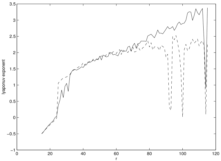
Figure 1:

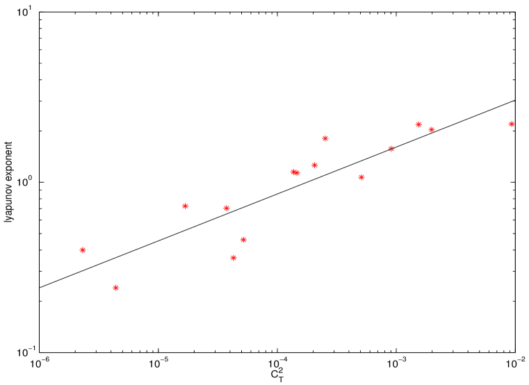
Figure 2: