Robustness of the noise-induced phase synchronization
in a general class of limit cycle oscillators

Abstract

We show that a wide class of uncoupled limit cycle oscillators can be in-phase synchronized by common weak additive noise. An expression of the Lyapunov exponent is analytically derived to study the stability of the noise-driven synchronizing state. The result shows that such a synchronization can be achieved in a broad class of oscillators with little constraint on their intrinsic property. On the other hand, the leaky integrate-and-fire neuron oscillators do not belong to this class, generating intermittent phase slips according to a power low distribution of their intervals.

Populations of nonlinear oscillators can be found in a variety of phenomena, including laser array wang88 , semiconductors hadley88wiesenfeld96 , chemical reactions kuramoto84 , society of living organisms winfree67winfree80 , and neurons gray89sompolinsky91 . In many of these systems, the phases of oscillations can precisely coincide owing to mutual interactions among oscillators. Alternatively, a strong periodic input may synchronize independent oscillators through the entrainment to the common input. In either cases, external or internal noise sources may disturb the phase synchronization, and therefore have long been considered to exert a negative influence on the precise temporal relationship between oscillators.

This view, however, has been challenged recently pikovsky84 ; pikovsky01 . Pikovsky studied, in his pioneering work, a population of circle maps stimulated by impulse inputs at discrete random times, and found that the common noise can induce stable phase synchronization. Since the noise-driven synchronization does not depend on the intrinsic frequency of oscillators, it differs from the entrainment to an external periodic input. Evidence is accumulating for the common noise-induced synchronization in several biological and physical systems. For instance, an ensemble of independent neuronal oscillators may be synchronized by a fluctuating input applied commonly to all of them. This is suggested by experimental studies of neural information coding mainen95 , in which the reproducibility of spike firing was tested for a repeated application of the same fluctuating or constant input current. Interestingly, the reproducibility of the output spike trains was much higher for the fluctuating input than for the constant one mainen95 ; tang97 ; jensen98ritt03kosmidis03 , indicating a high temporal precision of the spike responses to noisy input. In ecological systems, common environmental fluctuations such as climate changes may synchronize different populations separated by a large geographical distance royama92grenfell98 . In fluid dynamics, a common turbulent flow may generate a synchronized motion of floating particles yu90 .

All these findings indicate an active role of noise in synchronization of non-interacting dynamical elements. It remains, however, unclear whether the noise induced phase synchronization is specific to a limited class of oscillators, or can be generalized to a broad class of oscillators. In this study of a general class of limit-cycle oscillators, we show that common additive noise, even if it is weak, can induce phase synchronization regardless of their intrinsic properties and the initial conditions. Using the phase reduction method which is applicable to an arbitrary oscillator kuramoto84 , we analytically calculate the Lyapunov exponent of the synchronizing state and prove that the exponent is non-positive as long as the phase-dependent sensitivity is differentiable up to the second order. In addition, we investigate the scaling laws that appear in the dynamics of the relative phase when the perfect phase synchronization is deteriorated by a discontinuous phase-dependent sensitivity or oscillator-specific noise sources.

Population of $N$ identical nonlinear oscillators driven by common additive noise are described as

$$\dot{\bm{X}_{i}}=\bm{F}(\bm{X}_{i})+\bm{\xi}(t),$$ (1)

where $i=1,\cdots,N$ and $\bm{\xi}(t)$ is a vector of Gaussian white noise. The elements of the vector are normalized as $<\xi_{l}(t)>=0$ and $<\xi_{l}(t)\xi_{m}(s)>=2D_{lm}\delta(t-s)$, where $\bm{D}=(D_{lm})$ is a variance matrix of the noise components. Because all the oscillators are identical and do not interact with one another, we can study the phase synchronization of the entire population in a reduced system of two oscillators. Regarding the common noise as a weak perturbation to the deterministic oscillators, the phase reduction method gives the following dynamical equations of the phases:

$$\dot{\phi_{i}}=\omega+\bm{Z}(\phi_{i})\cdot\bm{\xi},$$ (2)

where $\omega$ is an intrinsic frequency of the unperturbed oscillators. $\bm{Z}$ is the phase-dependent sensitivity defined as $\bm{Z}(\phi)={\rm grad}_{\bm{X}}\phi|_{\bm{X}=\bm{X}_{0}(\phi)}$, where $\bm{X}_{0}(\phi)$ is the unperturbed limit cycle solution determined by $\bm{F}(\bm{X})$. We assume that $\bm{Z}$ is differentiable at least to the second order, although $\bm{Z}$ can be discontinuous for such oscillators that have discontinuous periodic solutions (e.g., integrate-and-fire neurons). As we will see later, the discontinuity of $\bm{Z}$ can significantly affect the noise-driven synchronization. To ensure the validity of the phase reduction, the weak noise must satisfy the condition $\omega\gg|D_{lm}|$.

Equation (2) implies that the synchronizing solution described as $\phi_{1}(t)=\phi_{2}(t)$ is absorbing, i.e., once two oscillators synchronize, they always remain synchronizing. Since the area of the phase space is limited ($0\leq\phi_{1},\phi_{2}<2\pi$), the phase variables starting from arbitrary initial phases can reach a neighborhood of the synchronizing solution with a finite probability in a finite time. To prove that the synchronizing solution is stable against perturbations, we analytically calculate the Lyapunov exponent $\lambda$ of the solution. We note that the stochastic equation (2) should be interpreted as a Stratonovich differential equation, since the phase reduction method assumes the conventional variable translations in differential equations. To remove the correlation between $\phi$ and $\bm{\xi}$, we translate Eq. (2) into an equivalent Ito differential equation stratonovich63horshemke84 :

$$\dot{\phi_{i}}=\omega+\bm{Z}^{\prime}(\phi_{i})\bm{D}\bm{Z}(\phi_{i})+\bm{Z}(\phi_{i})\cdot\bm{\xi},$$ (3)

where dash denotes differentiation with respect to $\phi$. Suppose that the two phases have an infinitesimally small difference $\psi=\phi_{2}-\phi_{1}$. Then, linearization of Eq. (3) with respect to $\psi$ gives

$$\dot{\psi}=[{\bm{(}}\bm{Z}^{\prime}(\phi)\bm{D}\bm{Z}(\phi){\bm{)}}^{\prime}+\bm{Z}^{\prime}(\phi)\cdot\bm{\xi}]\psi,$$ (4)

where $\phi$ obeys Eq. (3). By introducing a new variable $y=\log(\psi)$, Eq. (4) is further rewritten as

$$\dot{y}=(\bm{Z}^{\prime}\bm{D}\bm{Z})^{\prime}-(\bm{Z}^{\prime}\bm{D}\bm{Z}^{\prime})+\bm{Z}^{\prime}\cdot\bm{\xi}.$$ (5)

Since the Lyapunov exponent is defined as $\lim_{T\to\infty}(y(T)-y(0))/T$, the long time average of right hand side of Eq. (5) coincides with $\lambda$. Replacing the long time average with the ensemble average with respect to $\bm{\xi}$, we can represent $\lambda$ as

$$\lambda = <(\bm{Z}^{\prime}\bm{D}\bm{Z})^{\prime}-(\bm{Z}^{\prime}\bm{D}\bm{Z}^{\prime})+\bm{Z}^{\prime}\cdot\bm{\xi}>_{\xi}$$ (6)

$$= <(\bm{Z}^{\prime}\bm{D}\bm{Z})^{\prime}-(\bm{Z}^{\prime}\bm{D}\bm{Z}^{\prime})>_{\xi}$$

$$= \int_{0}^{2\pi}P_{st}(\phi)[(\bm{Z}^{\prime}\bm{D}\bm{Z})^{\prime}-(\bm{Z}^{\prime}\bm{D}\bm{Z}^{\prime})]d\phi.$$

Here, the second line follows from $<\bm{Z}^{\prime}(\phi)\cdot\bm{\xi}>_{\xi}=0$, which holds in Ito stochastic processes. $P_{st}$ is a steady distribution function of $\phi$ described as

$$P_{st}(\phi)=\frac{C}{Z^{2}(\phi)}\int_{\phi}^{\phi+2\pi}\exp{(V(x)-V(\phi))}dx,$$ (7)

with an effective potential $V(\phi)=-\int^{\phi}\frac{\omega+\bm{Z}^{\prime}(x)\bm{D}\bm{Z}(x)}{\bm{Z}(x)\bm{D}\bm{Z}(x)}dx$ and a normalization constant $C$. Fortunately under the assumption of weak noise, $\omega\gg|D_{lm}|$, $P_{st}$ is reduced to a constant function $P_{st}(\phi)=1/(2\pi)$. By substituting this into the last line of Eq. (6), and noting that the first term vanishes due to the periodicity of $\bm{Z}$, we finally obtain the following formula:

$$\lambda=-\frac{1}{2\pi}\int_{0}^{2\pi}\bm{Z}^{\prime}\bm{D}\bm{Z}^{\prime}d\phi\leq 0,$$ (8)

where the equality holds if $\bm{Z}$ is a constant function. Since the variance matrix is positive definite, $\lambda$ is non-positive. This implies that the phase synchronization induced by common noise is stable in an arbitrary oscillator system regardless of the detailed oscillatory dynamics, as long as $\bm{Z}$ is differentiable.

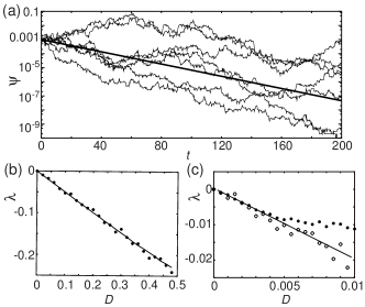
Figure 1: The common noise-induced phase synchronization. (a) The phase difference between two oscillators shows an exponential decay fluctuating around the theoretical behavior (solid line) derived from Eq.(8). Different curves correspond to different realizations of the random driving force $\xi(t)$. Here, $Z(\phi)=\sin{\phi}$, $\omega=1$ and $D=0.1$. (b) The Lyapunov exponent of the above synchronizing solution is shown as a function of the common-noise intensity (circles). The solid line shows an analytical result. (c) The Lyapunov exponent is calculated for the synchronizing solution of the Stuart-Landau oscillator. Numerical results are shown for both original (filled circles) and reduced (empty circles) oscillator systems. The solid line represents a theoretical result. The parameter values are set as $c_{0}=2$, $c_{2}=1$, $D_{11}=D_{22}=D$ and $D_{12}=D_{21}=0$.

To confirm the above analytical results, we numerically solve Eq. (2) to obtain the Lyapunov exponent for a specific choice of $Z$, i.e., $Z(\phi)=\sin(\phi)$. The phase difference between the two oscillators driven by common additive noise shows an exponential decay, and the decay constant well agrees with the analytical result (Fig. 1a). Consistent with equation (8), the magnitude of the negative Lyapunov exponent increases in proportion to the noise intensity $D$ (Fig. 1b). In order to confirm the validity of the phase reduction method, we employ the Stuart-Landau oscillators and compare the Lyapunov exponent derived from Eq. (8) with that calculated numerically in the original oscillator system (Fig. 1c). For the Stuart-Landau oscillator described as $\dot{A}=(1+ic_{0})A-(1+ic_{2})|A|^{2}A$, the phase sensitivity can be explicitly given as $Z(\phi)=(-c_{2}\cos{\omega\phi}-\sin{\omega\phi},-c_{2}\sin{\omega\phi}+\cos{\omega\phi})/\omega$, where $\omega=c_{0}-c_{2}$ kuramoto84 .

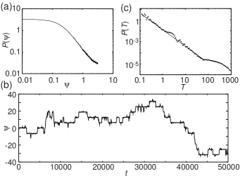
Figure 2: The intermittent phase slips induced by uncommon additive noise sources to the oscillators defined by $\omega=1$ and $Z(\phi)=\sin{\phi}$. The noise intensities $D=0.1$ and $d=0.001$. (a) The distribution of the phase difference over a sufficiently long time. (b) The time evolution of the phase difference exhibits intermittent phase slips. (c) The distribution of the inter-phase-slip intervals shows a power-low decay with an exponent of $-3/2$ (fitted by a solid line) and an exponential cutoff resulted from the additive noise term in Eq.(10).

In practical situations, the individual oscillators may be influenced by additional, oscillator-specific noise sources. They may appear from the fluctuations intrinsic in the oscillators, or a lack of perfect coincidences in the common driving noise. To discuss the influences of additional noise, Eq. (1) is modified to

$$\dot{\bm{X}_{i}}=\bm{F}(\bm{X}_{i})+\bm{\xi}(t)+\bm{\eta}_{i}(t),$$ (9)

where the uncommon noise sources $\bm{\eta}_{i}$ are normalized as $<\eta_{i,l}(t)>=0$ and $<\eta_{i,l}(t)\eta_{j,m}(s)>=2d_{lm}\delta_{ij}\delta(t-s)$. Linearization of Eq. (9) gives the stochastic equation of the phase difference as

$$\dot{\psi}=\left[{\bm{(}}\bm{Z}^{\prime}(\bm{D}+\bm{d})\bm{Z}{\bm{)}}^{\prime}+\bm{Z}^{\prime}\cdot(\bm{\xi}+\frac{\bm{\eta}_{1}+\bm{\eta}_{2}}{2})\right]\psi+\bm{Z}\cdot(\bm{\eta}_{2}-\bm{\eta}_{1}).$$ (10)

Since both multiplicative and additive factors fluctuate, Eq. (10) is regarded as a multiplicative stochastic process with additive noise, which has been studied in variety of fields kuramoto97anakao98teramae01 . The steady distribution function of Eq. (10) exhibits a power-low decay in a middle range of $\psi$ (Fig. 2a), implying that for most of the time the phases stay near phase synchronization even in the presence of uncommon noise sources. Simulations of Eq. (9) reveal that the system is trapped in the phase synchronizing state for certain intervals between intermittent phase slips (Fig. 2b). It is known that the intermittent bursts are characteristic to the stochastic processes driven simultaneously by multiplicative and additive noise sources cenya , and that the intervals between neighboring bursts obey a power low distribution with an exponent of $-3/2$. In Fig. 2c, the inter-slip intervals of the present phase dynamics obeys a power low distribution of the same exponent.

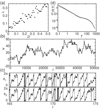
Figure 3: The unstable phase synchronization of integrate-and-fire models stimulated by a common noise source. The phase-dependent sensitivity of this oscillator is discontinuous, and the noise-driven synchronization is not ensured. $I=2$ and no uncommon noise, $d=0$. (a) The Lyapunov exponent $\lambda$ is plotted as a function of the common noise strength $D$. (b) The phase difference shows significant jitters, diffusing due to intermittent phase slips. Here and below, $D=0.1$. (c) The time evolution of the two phasess displays temporarily synchronizing ($t<170$) and desynchronizing ($t>170$) states. (d) The distribution of the inter-phase-slip intervals shows an exponential decay with an exponent of $-3/2$ (fitted by a solid line).

So far, we have assumed that the phase-dependent sensitivity $\bm{Z}$ is a continuous function of the phase. However, the phase reduction method does not ensure the continuity of $\bm{Z}$, and some oscillators do not have this property. For example, an integrate-and-fire neuron oscillator, which is described by $\dot{v}=I-v$ with a renewal condition $v(t)=1\to\lim_{\tau\to 0+}v(t+\tau)=0$, is frequently used for modeling neuronal activity, but it has the following discontinuous $\bm{Z}$:

$$Z(\phi)=\frac{\omega}{I}\exp{(\frac{\phi}{\omega})},~{}~{}0\leq\phi<2\pi,$$ (11)

where $\omega=2\pi/(\log{I}-\log{(I-1)})$. As shown in Fig. 3a, numerical integrations of Eq. (2) for the $\bm{Z}$ given in Eq. (11) show positive Lyapunov exponents, with the magnitudes increased with the intensity of the common noise. The phase difference does not decay exponentially, but fluctuates around the synchronizing state between the intermittent phase slips (Fig. 3b). Figure 3c displays the synchronized time evolution of the phase variables that is terminated by an abrupt phase slip at $t\approx 170$: After that, the two phases are desynchronized until they recover the phase synchronization (not shown). As in the previous case, the inter-slip intervals obey a $-3/2$ power-low distribution (Fig. 3d). This intermittency is essentially the same as the on-off intermittency of chaotic oscillators just before the onset of synchronization, thus associated with positive Lyapunov exponents fujisaka85fujisaka86 . Note that the discontinuity of the phase sensitivity and the resultant positive Lyapunov exponents are inherent in the leaky integrate-and-fire model. For example, the Hodgkin-Huxley model has a continuous and differentiable phase sensitivity, thus yielding a negative Lyapunov exponent and a stable phase synchronization in response to common noise (results not shown).

We briefly argue the relationships between the present study and two previous studies. In the stochastic resonance, the ability of an excitable system in detecting a weak signal can be optimized by noise of suitable intensity benzi81gammaitoni98 . The present study also argues the role of noise in improving the response reliability. However, here the improvement is achieved by the precise temporal coincidences between oscillators, whereas the stochastic resonance only enhances the response probability without caring the exact timing of events. Thus, the stability or Lyapunov exponent is not a central issue in the stochastic resonance, and the two studies deal with qualitatively different phenomena. Second, some chaotic oscillators exhibited phase synchronization when they were driven by common additive noise pikovsky01 ; zhou02 . However, it remained unknown whether this type of synchronization may appear in a broad class of, either chaotic or non-chaotic, oscillator systems. In this paper, we have proven that such a synchronization can be induced in a wide class of limit-cycle oscillators. A unified treatment of limit cycle oscillators and chaotic oscillators is awaited, as they may share many characteristic properties of the common noise-induced synchronization.

In conclusion, independent limit cycle oscillators can be synchronized by weak, common additive noise regardless of the detailed oscillatory dynamics and the initial phase distributions. The stability of this synchronizing solution only requires the presence of a second derivative of the phase-dependent sensitivity, so the solution can exist in a broad class of oscillators. The leaky integrate-and-fire oscillators do not belong to this class of oscillators, and show no perfect synchronization. The analytical evaluation of the Lyapunov exponent remains open for further studies for oscillators possessing non-differentiable phase sensitivity.

The authors are very grateful to T. Fukai for a critical reading of the manuscript and helpful comments. The authors thank T. Aoyagi, H. Nakao and Y. Tsubo for discussions. J.T. was supported by the 21st Century COE Program of Japanese Ministry of Education, Culture, Sprots, Science and Technology. D.T. acknowledges gratefully financial support by the Japan Society for Promotion of Science (JSPS). This work was partially supported by Grant-in-Aid for Scientific Research (B)(2) 16300096.

References

- (1) S. S. Wang and H. G. Winful, Appl. Phys. Lett. 52, 1774 (1988).
- (2) P. Hadley, M. R. Beasley and K. Wiesenfeld, Phys. Rev. B 38, 8712 (1988); K. Wiesenfeld, P. Colet and S. H. Strogatz, Phys. Rev. Lett. 76, 404 (1996).
- (3) Y. Kuramoto, Chemical Oscillation, Waves, and Turbulence (Springer-Verlag, Tokyo, 1984); (Dover Edition, 2003).
- (4) A. T. Winfree, J. Theor. Biol. 16 (1967), 15; A. T. Winfree, The Geometry of Biological Time (Springer, New York, 1980).
- (5) C. M. Gray, P. König, A. K. Engel and W. Singer, Nature 338, 334 (1989); H. Sompolinsky, D. Golomb and D. Kleinfeld, Phys. Rev. A 43, 6990 (1991).
- (6) A. S. Pikovsky, In R. Z. Sagdeev, Editor, Nonlinear and Turbulent Processes in Physics, 1601, (Harwood, Singapore, 1984).
- (7) A. S. Pikovsky, M. Rosenblum, and J. Kurths, Synchronization -A Unified Approach to Nonlinear Science (Cambridge University Press, Chambridge, U.K., 2001).
- (8) Z. F. Mainen and T. J. Sejnowski Sience 268, 1503 (1995).
- (9) A. C. Tang, A. M. Bartels and T. J. Sejnowski, Cerebral Cortex 7, 502 (1997).
- (10) R. V. Jensen, Phys. Rev. E 58, R6907 (1998); J. Ritt, Phys. Rev. E 68, 041915 (2003); E. K. Kosmidis and K. Pakdaman, J. Comput. Neurosci. 14, 5 (2003).
- (11) T. Royama, Analycal Population Dynamics (Chapman and Hall, London, 1992); B. T. Brenfell et al., Nature, 394, 674 (1998).
- (12) L. Yu, E. Ott, and Q. Chen, Phys. Rev. Lett. 65, 2935 (1990).
- (13) R. L. Stratonovich, Topics in the Theory of Random Noise (Gordon and Breach, New York, 1963); W. Horshemke and R. Lefever, Noise-Induced Transitions (Springer-Verlag, Berlin, 1984).
- (14) Y. Kuramoto and H. Nakao, Phys. Rev. Lett. 78, 4039 (1997); H. Nakao, Phys. Rev. E 58, 1591 (1998); J. Teramae and Y. Kuramoto, Phys. Rev. E 63, 036210 (2001).
- (15) A. Čenya, A. N. Angnostopoulos, and G. L. Bleris, Pys. Lett. A 224, 346 (1997).
- (16) H. Fujisaka and H. Yamada, Prog. Theor. Phys. 74, 918 (1985); H. Fujisaka and H. Yamada, Prog. Theor. Phys. 75, 1087 (1986).
- (17) R. Benzi, A. Sutera and A. Vulpiani, J. Phys. A 14, L453 (1981); L. Gammaitoni, P. Hänggi, P. Jung and F. Marchesoni, Rev. Mod. Phys. 70, 223 (1998); T. Fukai, Neuroreport 11, 3457 (2000).
- (18) C. Zhou, J. Kurths, Phys. Rev. Lett. 88, 230602 (2002).