Bose-Einstein Condensates in Superlattices

Abstract

We consider the Gross-Pitaevskii (GP) equation in the presence of periodic and quasiperiodic superlattices to study cigar-shaped Bose-Einstein condensates (BECs) in such potentials. We examine spatially extended wavefunctions in the form of modulated amplitude waves (MAWs). With a coherent structure ansatz, we derive amplitude equations describing the evolution of spatially modulated states of the BEC. We then apply second-order multiple scale perturbation theory to study harmonic resonances with respect to a single lattice wavenumber as well as ultrasubharmonic resonances that result from interactions of both wavenumbers of the superlattice. In each case, we determine the resulting system’s equilibria, which represent spatially periodic solutions, and subsequently examine the stability of the corresponding solutions by direct simulations of the GP equation, identifying them as typically stable solutions of the model. We then study subharmonic resonances using Hamiltonian perturbation theory, tracing robust, spatio-temporally periodic patterns.

PACS: 05.45.-a, 03.75.Lm, 05.30.Jp, 05.45.Ac

MSC: 37N20, 35Q55, 81V45

Keywords: Bose-Einstein condensates, multiple-scale perturbation theory, Hamiltonian systems

1 Introduction

At very low temperatures, particles in a dilute bose gas can occupy the same quantum (ground) state, forming a Bose-Einstein condensate (BEC) [48, 21, 30, 17], which appears as a sharp peak (over a broader distribution) in both coordinate and momentum space. As the gas is cooled, condensation (of a large fraction of the atoms in the gas) occurs via a quantum phase transition, emerging when the wavelengths of individual atoms overlap and behave identically. Atoms of mass $m$ and temperature $T$ constitute quantum wavepackets whose spatial extent is given by the de Broglie wavelength

$$\lambda_{db}=\sqrt{\frac{2\pi\hbar^{2}}{mk_{B}T}}\,,$$ (1)

which represents the uncertainty in position associated with the momentum distribution [30] (where $\hbar$ is Planck’s constant and $k_{B}$ is Boltzmann’s constant). The atomic wavepackets overlap once atoms are cooled sufficiently so that $\lambda_{db}$ is comparable to the separation between atoms, as bosonic atoms then undergo a quantum phase transition to form a BEC (a coherent cloud of atoms). Although a condensate constitutes a quantum phenomenon, such “matter waves” can often be observed macroscopically, with the number of condensed atoms $N$ ranging from several thousand (or less) to several million (or more) [21].

BECs were first observed experimentally in 1995 in dilute alkali gases such as vapors of rubidium and sodium [4, 22]. In these experiments, atoms were confined in magnetic traps, evaporatively cooled to a fraction of a microkelvin, left to expand by switching off the confining trap, and subsequently imaged with optical methods. A sharp peak in the velocity distribution was observed below a critical temperature, indicating that condensation had occured [as the alkali atoms were now condensed in the same (ground) state]. Under the typical confining conditions of experimental settings, BECs are inhomogeneous, so condensates arise as a narrow peak not only in momentum space but also in coordinate space.

The macroscopic observability of the condensates in coordinate and momentum space has led to novel methods of investigating quantities such as energy and density distributions, interference phenomena, the frequencies of collective excitations, the temperature dependence of BECs, among others [21] (for comprehensive reviews, the interested reader should consult Refs. [48, 57]). Another consequence of this inhomogeneity is that the effects of two-body interactions are greatly enhanced, despite the fact that bose gases are extremely dilute (with the average distance between atoms typically more than ten times the range of interatomic forces). For example, these interactions reduce the condensate’s central density and enlarge the size of the condensate cloud, which becomes macroscopic and can be measured directly with optical imaging methods.

BECs have two characteristic length scales. The condensate density varies on the scale of the harmonic oscillator length $a_{ho}=\sqrt{\hbar/(m\omega_{ho})}$ [which is typically on the order of a few microns], where $\omega_{ho}=(\omega_{x}\omega_{y}\omega_{z})^{1/3}$ is the geometric mean of the trapping frequencies. The “coherence length” (or “healing length”), determined by balancing the quantum pressure and the condensate’s interaction energy, is $\chi=1/\sqrt{8\pi|a|\bar{n}}$ [and is also typically of the order of a few microns], where $\bar{n}$ is the mean particle density and $a$, the (two-body) $s$-wave scattering length, is determined by the atomic species of the condensate. Interactions between atoms are repulsive when $a>0$ and attractive when $a<0$. For a dilute ideal gas, $a\approx 0$. The length scales in BECs should be contrasted with those in systems like superfluid helium, in which the effects of inhomogeneity occur on a microscopic scale fixed by the interatomic distance [21].

If considering only two-body, mean-field interactions, a dilute Bose-Einstein gas near zero temperature can be modeled using a cubic nonlinear Schrödinger equation (NLS) with an external potential, which is also known as the Gross-Pitaevskii (GP) equation. This is written [21]

$$i\hbar{\Psi}_{t}=\left(-\frac{\hbar^{2}\nabla^{2}}{2m}+g_{0}|\Psi|^{2}+{\mathcal{V}}(\vec{r})\right)\Psi\,,$$ (2)

where $\Psi=\Psi(\vec{r},t)$ is the condensate wave function normalized to the number of atoms, ${\mathcal{V}}(\vec{r})$ is the external potential, and the effective interaction constant is $g_{0}=[4\pi\hbar^{2}a/m][1+O(\zeta^{2})]$, where $\zeta\equiv\sqrt{|\Psi|^{2}|a|^{3}}$ is the dilute-gas parameter [21, 35, 7].

BECs are modeled in the quasi-one-dimensional (quasi-1D) regime when the transverse dimensions of the condensate are on the order of its healing length and its longitudinal dimension is much larger than its transverse ones [13, 14, 12, 21]. In this regime, one employs the 1D limit of a 3D mean-field theory (generated by averaging in the transverse plane) rather than a true 1D mean-field theory, which would be appropriate were the transverse dimension on the order of the atomic interaction length or the atomic size [13, 55, 8]. The resulting 1D equation is [55, 21]

$$i\hbar u_{t}=-[\hbar^{2}/(2m)]u_{xx}+g|u|^{2}u+V(x)u\,,$$ (3)

where $u$, $g$, and $V$ are, respectively, the rescaled 1D wave function (“order parameter”), interaction constant, and external trapping potential. The quantity $|u|^{2}$ gives the atomic number density. The self-interaction parameter $g$ is tunable (even its sign), because the scattering length $a$ can be adjusted using magnetic fields in the vicinity of a Feshbach resonance [24, 34]. The manipulation of Feshbach resonances has become one of the most active areas in the study of ultracold atoms, as (for example) numerous research groups are investigating the intermediate regime between molecular condensates and degenerate Fermi gases (the so-called “BEC-BCS” crossover regime). Theoretical algorithms for manipulating $a$, such as alternating it periodically between positive and negative values, have been developed by analogy with “dispersion management” in nonlinear optics.

In forming a BEC, the atoms are trapped using a confining magnetic or optical potential $V(x)$, which is then turned off so that the gas can expand and be imaged. In early experiments, only parabolic (“harmonic”) potentials were employed, but a wide variety of potentials can now be constructed experimentally. In addition to harmonic traps, these include double-well traps (see, e.g., [5] and references therein), periodic lattices (see, e.g., [11] for a review), and superlattices [47, 54] (which can be either periodic or quasiperiodic), and superpositions of lattices or superlattices with harmonic traps. Optical lattices and superlattices are created using counter-propagating laser beams, and higher-dimensional versions of many of the aforementioned potentials have also been achieved experimentally.

The existence of quasi-1D (“cigar-shaped”) BECs motivates the study of lower dimensional models such as Eq. (3). The case of periodic and quasiperiodic potentials without a confining trap along the longitudinal dimension of the lattice is of particular theoretical and experimental interest. Such potentials have been used, for example, to study Josephson effects [3], squeezed states [45], Landau-Zener tunneling and Bloch oscillations [42], and the transition between superfluidity and Mott insulation at both the classical [56, 19] and quantum [28] levels. Moreover, with each lattice site occupied by one alkali atom in its ground state, BECs in optical lattices show promise as a register in a quantum computer [52, 58].

In experiments, a weak harmonic trap is typically used on top of the optical lattice (OL) or optical superlattice (OSL) to prevent the particles from escaping. The lattice is also generally turned on after the trap. If one wishes to include the trap in theoretical analyses, then $V(x)$ is modeled by

$$V(x)=V_{1}\cos(\kappa_{1}x)+V_{2}\cos(\kappa_{2}x)+V_{h}x^{2}\,,$$ (4)

where $\kappa_{1}$ is the primary lattice wavenumber, $\kappa_{2}>\kappa_{1}$ is the secondary lattice wavenumber, $V_{1}$ and $V_{2}$ are the associated lattice amplitudes, and $V_{h}$ represents the magnitude of the harmonic trap. Note that $V_{1}$, $V_{2}$, $V_{h}$, $\kappa_{1}$, and $\kappa_{2}$ can all be tuned experimentally, so that the external potential’s length scales are easily manipulated. The sinusoidal terms in (4) dominate for small $x$, but the harmonic trap otherwise becomes quickly dominant. When $V_{h}\ll V_{1}\,,V_{2}$, the potential is dominated by its periodic (or quasiperiodic) contributions for many periods [18, 50]. BECs in OLs with up to $200$ wells have been created experimentally [46].

In this work, we let $V_{h}=0$ and focus on OL and OSL potentials. Spatially periodic potentials have been employed in experimental studies of BECs [29, 3, 45, 42, 28, 52] and have also been studied theoretically [13, 10, 20, 41, 2, 39, 40, 43, 49, 56, 38, 33]; see also the recent reviews [32, 31]. In experiments reported in 2003, BECs were loaded into OSLs with $\kappa_{2}=3\kappa_{1}$ [47]. However, there has thus far been very little theoretical research on BECs in superlattice potentials [54, 23, 37, 25]. In this work, we consider both periodic (rational $\kappa_{2}/\kappa_{1}$) and quasiperiodic (irrational $\kappa_{2}/\kappa_{1}$) OSLs.

We focus here on spatially extended solutions rather than on localized waves (solitons). For BECs loaded into OSLs, the interest in such extended wavefunctions is twofold. First, BECs were successfully loaded into OSL potentials in recent experiments [47] (in which extended solutions were observed). Second, MAWs in BECs in OSLs can be used to study period-multiplied states and generalizations thereof [49, 50, 51].

On the first front, ⁸⁷Rb atoms were loaded into an OSL by the sequential creation of two lattice structures. The atoms were initially loaded into every third site of an OL. A second periodic structure was subsequently added so that the atoms could be transferred from long-period lattice sites to corresponding short-period lattice sites in a patterned loading.

On the second front, Machholm et al. [39] studied period-doubled states (in $|u|^{2}$), interpreting them as soliton trains to attempt to explain experimental studies by Cataliottiet al. [19], who observed superfluid current disruption in chains of weakly coupled BECs in OL potentials. More recently, experimental observations of period doubled wavefunctions in BECs in OL potentials have now been reported [26]. From a dynamical systems perspective, period-multiplied states arise at the center of KAM islands in phase space; the location and size of these islands have been estimated using Hamiltonian perturbation theory and multiple scale analysis [49, 50, 51].

In this study, we investigate spatially extended solutions of BECs in periodic and quasiperiodic OSLs. We apply a coherent structure ansatz to Eq. (3), yielding a parametrically forced Duffing equation describing the spatial evolution of the field. We employ second-order multiple scale perturbation theory to study its periodic orbits (called “modulated amplitude waves” and denoted MAWs), and illustrate their dynamical stability with numerical simulations of the GP equation. We consider harmonic ($1\!:\!1$) resonances and two types of ultrasubharmonic resonances—resulting from, respectively, “additive” ($2\!:\!1+1$) and “subtractive” ($2\!:\!1-1$) interactions—all of which arise at the $O(\varepsilon^{2})$ level of analysis. Because ultrasubharmonic resonances result from the interaction of multiple superlattice wavenumbers, they cannot occur in BECs loaded into regular OLs. We then explore subharmonic resonances using Hamiltonian perturbation theory, identifying various relevant patterns including quasi-stationary ones (with weak amplitude oscillations) and spatio-temporally breathing ones (see the details below).

We structure the rest of our presentation as follows: We first introduce modulated amplitude waves and use multiple scale perturbation theory to derive “slow flow” dynamical equations that describe the resonance phenomena under consideration. We analyze these equations and corroborate our results and test the stability of the MAWs with direct numerical simulations of the GP equation. We then examine subharmonic resonances using Hamiltonian perturbation theory and additional numerics. Finally, we summarize our findings and present our conclusions.

2 Modulated Amplitude Waves

To study MAWs, we employ the ansatz

$$u(x,t)=R(x)\exp\left(i\left[\theta(x)-\mu t\right]\right)\,.$$ (5)

When these (temporally periodic) coherent structures (5) are also spatially periodic, they are called modulated amplitude waves (MAWs) [16, 15]. The orbital stability of MAWs for the cubic NLS with elliptic potentials has been studied by Bronski et al [13, 12, 14]. To obtain stability information about sinusoidal potentials, one takes the limit as the elliptic modulus $k$ approaches zero [36]. When $V(x)$ is periodic, the resulting MAWs generalize the Bloch modes that occur in the theory of linear systems with periodic potentials [53, 6, 38, 10, 20]. In this work, we extend recent studies [49, 50] of the dynamical behavior of MAWs of BECs in lattice potentials to superlattice potentials.

Inserting Eq. (5) into Eq. (3), equating the real and imaginary components of the resulting equation, and defining $S:=R^{\prime}$ yields the following two-dimensional system of nonlinear ordinary differential equations:

$$R^{\prime} =S\,,$$

$$S^{\prime} =\frac{c^{2}}{R^{3}}-\frac{2m\mu R}{\hbar}+\frac{2mg}{\hbar^{2}}R^{3}+\frac{2m}{\hbar^{2}}V(x)R\,.$$

The parameter $c$ is given by the relation

$$\theta^{\prime}(x)=\frac{c}{R^{2}}\,,$$ (6)

which indicates conservation of “angular momentum” [13]. Constant phase solutions (i.e., standing waves), which constitute an important special case, satisfy $c=0$. In the rest of the paper, we restrict ourselves to this class of solutions, so that

$$R^{\prime} =S\,,$$

$$S^{\prime} =-\frac{2m\mu R}{\hbar}+\frac{2mg}{\hbar^{2}}R^{3}+\frac{2m}{\hbar^{2}}V(x)R\,.$$ (7)

We consider the case with $V_{h}=0$ (which implies, in practice, that the harmonic trap is negligible with respect to the OSL potential for the domain of interest) and define

$$\tilde{\delta}:=\frac{2m\mu}{\hbar}\,,\quad\varepsilon\tilde{\alpha}:=-\frac{2mg}{\hbar^{2}}\,,\quad\tilde{V}(x):=-\frac{2m}{\hbar^{2}}V(x)\,,$$ (8)

where

$$\tilde{V}(x)=\varepsilon[\tilde{V}_{1}\cos(\kappa_{1}x)+\tilde{V}_{2}\cos(\kappa_{2}x)]\,,$$ (9)

the parameters $\tilde{\delta}$, $\tilde{\alpha}$, and $\tilde{V}_{j}$ are $O(1)$ quantities, and the lattice wavenumbers $\kappa_{j}$ can either be commensurate (rational multiples of each other) or incommensurate, so that the OSL can be, respectively, either periodic or quasiperiodic. We let $\kappa_{2}>\kappa_{1}$ without loss of generality, so that $\kappa_{1}$ is the primary lattice wavenumber. In our numerical simulations, we focus on the case $\kappa_{2}=3\kappa_{1}$ which has been achieved experimentally [47].

For notational convenience, we drop the tildes from $\tilde{\delta}$, $\tilde{\alpha}$, and $\tilde{V}_{j}$, so that Eq. (7) is written

$$R^{\prime\prime}+\delta R+\varepsilon\alpha R^{3}+\varepsilon R[V_{1}\cos(\kappa_{1}x)+V_{2}\cos(\kappa_{2}x)]=0\,.$$ (10)

In this paper, we consider the case $\delta>0$ corresponding to a positive chemical potential.

3 Multiple Scale Perturbation Theory and Spatial Resonances

To employ multiple scale perturbation theory [9, 53], we define “slow space” $\eta:=\varepsilon x$ and “stretched space”

$$\xi:=bx=[1+\varepsilon b_{1}+\varepsilon^{2}b_{2}+O(\varepsilon^{3})]x\,.$$ (11)

We then expand the wavefunction amplitude $R$ in a power series,

$$R=R_{0}+\varepsilon R_{1}+\varepsilon^{2}R_{2}+O(\varepsilon^{3})\,,$$ (12)

and stretch the spatial dependence in the OSL potential, which is then written

$$\bar{V}(\xi)=V_{1}\cos(\kappa_{1}\xi)+V_{2}\cos(\kappa_{2}\xi)\,.$$ (13)

Inserting these expansions, Eq. (10) becomes

$$\left[1+b_{1}\varepsilon+b_{2}\varepsilon^{2}+O(\varepsilon^{3})\right]^{2}\left[\frac{\partial^{2}R_{0}}{\partial\xi^{2}}+\varepsilon\frac{\partial^{2}R_{1}}{\partial\xi^{2}}+\varepsilon^{2}\frac{\partial^{2}R_{2}}{\partial\xi^{2}}+O(\varepsilon^{3})\right]$$

$$\qquad+2\varepsilon\left[1+b_{1}\varepsilon+b_{2}\varepsilon^{2}+O(\varepsilon^{3})\right]\left[\frac{\partial^{2}R_{0}}{\partial\xi\partial\eta}+\varepsilon\frac{\partial^{2}R_{1}}{\partial\xi\partial\eta}+\varepsilon^{2}\frac{\partial^{2}R_{2}}{\partial\xi\partial\eta}+O(\varepsilon^{3})\right]$$

$$\qquad+\varepsilon^{2}\left[\frac{\partial^{2}R_{0}}{\partial\eta^{2}}+\varepsilon\frac{\partial^{2}R_{1}}{\partial\eta^{2}}+\varepsilon^{2}\frac{\partial^{2}R_{2}}{\partial\eta^{2}}+O(\varepsilon^{3})\right]$$

$$\qquad+\delta\left[R_{0}+\varepsilon R_{1}+\varepsilon^{2}R_{2}+O(\varepsilon^{3})\right]+\varepsilon\alpha\left[R_{0}+\varepsilon R_{1}+\varepsilon^{2}R_{2}+O(\varepsilon^{3})\right]^{3}$$

$$\qquad+\varepsilon\left[R_{0}+\varepsilon R_{1}+\varepsilon^{2}R_{2}+O(\varepsilon^{3})\right]\left[V_{1}\cos(\kappa_{1}\xi)+V_{2}\cos(\kappa_{2}\xi)\right]=0\,.$$ (14)

To perform multiple scale analysis, we equate the coefficients of terms of different order (in $\varepsilon$) in turn. At $O(1)=O(\varepsilon^{0})$, we obtain

$$\frac{\partial^{2}R_{0}}{\partial\xi^{2}}+\delta R_{0}=0\,,$$

which has the solution

$$R_{0}(\xi,\eta)=A(\eta)\cos(\sqrt{\delta}\xi)+B(\eta)\sin(\sqrt{\delta}\xi)\,,$$ (15)

for slowly-varying amplitudes $A(\eta)$, $B(\eta)$, equations of motion for which arise at $O(\varepsilon)$.

Equating coefficients at $O(\varepsilon)$ yields

$$\frac{\partial^{2}R_{1}}{\partial\xi^{2}}+\delta R_{1} =\left[2b_{1}\delta A-2\sqrt{\delta}B^{\prime}-\frac{3}{4}\alpha A(A^{2}+B^{2})\right]\cos(\sqrt{\delta}\xi)$$

$$\quad+\left[2b_{1}\delta B+2\sqrt{\delta}A^{\prime}-\frac{3}{4}\alpha B(A^{2}+B^{2})\right]\sin(\sqrt{\delta}\xi)$$

$$\quad+\frac{\alpha A}{4}[-A^{2}+3B^{2}]\cos(3\sqrt{\delta}\xi)+\frac{\alpha B}{4}[-3A^{2}+B^{2}]\sin(3\sqrt{\delta}\xi)$$

$$\quad+\frac{V_{1}A}{2}\cos([\kappa_{1}-\sqrt{\delta}]\xi)+\frac{V_{1}A}{2}\cos([\kappa_{1}+\sqrt{\delta}]\xi)$$

$$\quad-\frac{V_{1}B}{2}\sin([\kappa_{1}-\sqrt{\delta}]\xi)+\frac{V_{1}B}{2}\sin([\kappa_{1}+\sqrt{\delta}]\xi)$$

$$\quad+\frac{V_{2}A}{2}\cos([\kappa_{2}-\sqrt{\delta}]\xi)+\frac{V_{2}A}{2}\cos([\kappa_{2}+\sqrt{\delta}]\xi)$$

$$\quad-\frac{V_{2}B}{2}\sin([\kappa_{2}-\sqrt{\delta}]\xi)+\frac{V_{2}B}{2}\sin([\kappa_{2}+\sqrt{\delta}]\xi)\,.$$ (16)

For $R_{1}(\xi,\eta)$ to be bounded, the coefficients of the secular terms in Eq. (16) must vanish [53, 9]. The harmonics $\cos(\sqrt{\delta}\xi)$ and $\sin(\sqrt{\delta}\xi)$ are always secular, whereas $\cos(3\sqrt{\delta}\xi)$ and $\sin(3\sqrt{\delta}\xi)$ are never secular. The other harmonics are secular only in the case of $2\!:\!1$ subharmonic resonances [49, 50], which can occur with respect to either the primary ($\kappa_{1}=2\sqrt{\delta}$) or secondary ($\kappa_{2}=2\sqrt{\delta}$) wavenumber of the lattice. We will consider the situation in which (16) is non-resonant and turn our attention to other resonant situations at $O(\varepsilon^{2})$ that arise from interactions between both lattice wavenumbers. [Our $O(\varepsilon^{2})$ analysis below can be repeated in the presence of $2\!:\!1$ resonances.] At $O(\varepsilon)$, one obtains either no resonance, a long-wavelength subharmonic resonance, or a short-wavelength subharmonic resonance.

Equating the coefficients of the secular terms to zero in Eq. (16) yields the following equations of motion describing the slow dynamics:

$$A^{\prime} =-b_{1}\sqrt{\delta}B+\frac{3\alpha}{8\sqrt{\delta}}B(A^{2}+B^{2})\,,$$

$$B^{\prime} =b_{1}\sqrt{\delta}A-\frac{3\alpha}{8\sqrt{\delta}}A(A^{2}+B^{2})\,.$$ (17)

We convert (17) to polar coordinates with $A(\eta)=C\cos[\varphi(\eta)]$ and $B(\eta)=C\sin[\varphi(\eta)]$ and see immediately that each circle of constant $C$ is invariant. The dynamics on each circle is given by

$$\varphi(\eta)=\varphi(0)+\left[b_{1}\sqrt{\delta}-\frac{3\alpha}{8\sqrt{\delta}}C^{2}\right]\eta\,.$$ (18)

We examine the special circle of equilibria, corresponding to periodic orbits of (3), which satisfies

$$C^{2}=A^{2}+B^{2}=\frac{8b_{1}\delta}{3\alpha}\,.$$ (19)

We are interested in the $O(\varepsilon^{2})$ effects, which we now analyze. At this second order of perturbation theory, BECs in OSL potentials exhibit dynamical behavior that cannot occur in BECs in simpler OL potentials (where, for example, solutions of type of Eq. (19) straightforwardly arise [51]).

Equating coefficients at $O(\varepsilon^{2})$ yields

$$\frac{\partial^{2}R_{2}}{\partial\xi^{2}}+\delta R_{2} =-(b_{1}^{2}+2b_{2})\frac{\partial^{2}R_{0}}{\partial\xi^{2}}-\frac{\partial^{2}R_{0}}{\partial\eta^{2}}-2b_{1}\frac{\partial^{2}R_{0}}{\partial\xi\partial\eta}-3\alpha R_{0}^{2}R_{1}-2b_{1}\frac{\partial^{2}R_{1}}{\partial\xi^{2}}-2\frac{\partial^{2}R_{1}}{\partial\xi\partial\eta}$$

$$\quad-R_{1}V_{1}\cos(\kappa_{1}\xi)-R_{2}V_{2}\cos(\kappa_{2}\xi)\,,$$ (20)

where one inserts the expressions for $R_{0}$, $R_{1}$, and their derivatives into the right-hand-side of (20).

To find the secular terms in Eq. (20), we compute

$$R_{1}(\xi,\eta) =C(\eta)\cos(\sqrt{\delta}\xi)+D(\eta)\sin(\sqrt{\delta}\xi)+R_{1p}(\xi,\eta)\,,$$

$$R_{1p}(\xi,\eta) =c_{1}\cos(3\sqrt{\delta}\xi)+c_{2}\sin(3\sqrt{\delta}\xi)$$

$$\quad+\sum_{j=1}^{2}\left[c_{3}^{j}\cos([\kappa_{j}-\sqrt{\delta}]\xi)+c_{4}^{j}\cos([\kappa_{j}+\sqrt{\delta}]\xi)+c_{5}^{j}\sin([\kappa_{j}-\sqrt{\delta}]\xi)+c_{6}^{j}\sin([\kappa_{j}+\sqrt{\delta}]\xi)\right]\,,$$ (21)

where $j\in\{1\,,2\}$ and

$$c_{1} =\frac{\alpha}{32\delta}A(A^{2}-3B^{2})\,,\quad c_{2}=\frac{\alpha}{32\delta}B(3A^{2}-B^{2})\,,$$

$$c_{3}^{j} =\frac{V_{j}A}{2\kappa_{j}(\kappa_{j}-2\sqrt{\delta})}\,,\quad c_{4}^{j}=\frac{V_{j}A}{2\kappa_{j}(\kappa_{j}+2\sqrt{\delta})}\,,$$

$$c_{5}^{j} =\frac{V_{j}B}{2\kappa_{j}(\kappa_{j}-2\sqrt{\delta})}\,,\quad c_{6}^{j}=\frac{V_{j}B}{2\kappa_{j}(\kappa_{j}+2\sqrt{\delta})}\,.$$ (22)

Inserting (15) and (21) into Eq. (20) and expanding the resulting equation trigonometrically yields $19$ harmonics (that are also present for sines), which we list in Table 1. We indicate which of these harmonics are always secular, sometimes secular, and never secular.

At this order of perturbation theory, one finds $2\!:\!1$ (primary subharmonic), $4\!:\!1$ (secondary subharmonic), $1\!:\!1$ (harmonic), $2\!:\!1\!+\!1$ (additive ultrasubharmonic), and $2\!:\!1\!-\!1$ (subtractive ultrasubharmonic) resonances. The first three types of resonances can occur with respect to either $\kappa_{1}$ or $\kappa_{2}$, whereas the latter two require the interaction of both superlattice wavenumbers. Harmonic and ultrasubharmonic spatial resonances have not been analyzed previously for BECs, and subharmonic resonances have only been analyzed in the case of regular OL potentials. At $O(\varepsilon)$, we considered the case without $2\!:\!1$ resonances, so the associated resonance conditions ($\kappa_{j}=\pm 2\sqrt{\delta}$) are necessarily not satisfied at the present [$O(\varepsilon^{2})$] stage, as indicated in Table 1. Second-order subharmonic ($4\!:\!1$) resonances have been studied in BECs in regular OL potentials [49, 50]. Their associated resonance conditions are $\kappa_{j}=\pm 4\sqrt{\delta}$. (We return to subharmonic resonances in the case of OSLs later when we apply Hamiltonian perturbation theory.) The resonance relations for harmonic resonances are $\kappa_{j}=\pm\sqrt{\delta}$. We will consider solutions that have harmonic resonance with respect to the primary lattice wavenumber $\kappa_{1}$. The resonance relation for additive ultrasubharmonic resonances is $\kappa_{2}+\kappa_{1}=\pm 2\sqrt{\delta}$, and that for subtractive ultrasubharmonic resonances is $\kappa_{2}-\kappa_{1}=\pm 2\sqrt{\delta}$. In the remainder of this section, we consider the non-resonant, harmonically resonant, and the two types of ultrasubharmonic resonant states in turn.

It is also important to remark that with the slow spatial variable $\eta=\varepsilon x$, the approximate solutions $R(x)$ obtained perturbatively are valid for $|x|\lesssim O(\varepsilon^{-1})$ despite the fact that we employ a second-order multiple scale expansion. By incorporating a third (“super slow”) scale $\varepsilon^{2}x$, which is more technically demanding, one can obtain approximate solutions that are valid for $|x|\lesssim O(\varepsilon^{-2})$ [9].

Label Harmonic Secular? Resonance when secular 1 $\cos(\sqrt{\delta}\xi)$ Yes N/A 2 $\cos(3\sqrt{\delta}\xi)$ No N/A 3 $\cos(5\sqrt{\delta}\xi)$ No N/A 4 $\cos([\kappa_{1}-\sqrt{\delta}]\xi)$ Assumed not in resonance at $O(\varepsilon)$ $2\!:\!1$ 5 $\cos([\kappa_{1}+\sqrt{\delta}]\xi)$ Assumed not in resonance at $O(\varepsilon)$ $2\!:\!1$ 6 $\cos([\kappa_{2}-\sqrt{\delta}]\xi)$ Assumed not in resonance at $O(\varepsilon)$ $2\!:\!1$ 7 $\cos([\kappa_{2}+\sqrt{\delta}]\xi)$ Assumed not in resonance at $O(\varepsilon)$ $2\!:\!1$ 8 $\cos([\kappa_{1}-3\sqrt{\delta}]\xi)$ Sometimes $4\!:\!1$ 9 $\cos([\kappa_{1}+3\sqrt{\delta}]\xi)$ Sometimes $4\!:\!1$ 10 $\cos([\kappa_{2}-3\sqrt{\delta}]\xi)$ Sometimes $4\!:\!1$ 11 $\cos([\kappa_{2}+3\sqrt{\delta}]\xi)$ Sometimes $4\!:\!1$ 12 $\cos([2\kappa_{1}-\sqrt{\delta}]\xi)$ Sometimes $1\!:\!1$ 13 $\cos([2\kappa_{1}+\sqrt{\delta}]\xi)$ Sometimes $1\!:\!1$ 14 $\cos([2\kappa_{2}-\sqrt{\delta}]\xi)$ Sometimes $1\!:\!1$ 15 $\cos([2\kappa_{2}+\sqrt{\delta}]\xi)$ Sometimes $1\!:\!1$ 16 $\cos([\kappa_{1}+\kappa_{2}-\sqrt{\delta}]\xi)$ Sometimes $2\!:\!1\!+\!1$ 17 $\cos([\kappa_{1}+\kappa_{2}+\sqrt{\delta}]\xi)$ Sometimes $2\!:\!1\!+\!1$ 18 $\cos([\kappa_{1}-\kappa_{2}-\sqrt{\delta}]\xi)$ Sometimes $2\!:\!1\!-\!1$ 19 $\cos([\kappa_{1}-\kappa_{2}+\sqrt{\delta}]\xi)$ Sometimes $2\!:\!1\!-\!1$

Table 1: The harmonics in the right-hand-side of Eq. (20) after the formulas for $R_{0}$ (15) and $R_{1}$ (21) are inserted. We only list the cosines in this table, but the sines of these harmonics are present as well. We designate which harmonics are always secular, sometimes secular (under an appropriate resonance condition, as detailed in the text), and never secular.

Before proceeding, we also remark that in light of KAM theory, one expects different dynamical behavior (at least mathematically) depending on whether $\kappa_{2}/\kappa_{1}$ is an integer, a rational number, or an irrational number. Only the situation $\kappa_{2}=3\kappa_{1}$ has been prepared experimentally, so we concentrate on that case in our numerical simulations.

We note additionally that we simulated the dynamics and examined the stability of MAWs using a numerical domain with periodic boundary conditions. This allows us to handle integer or rational values of $\kappa_{2}/\kappa_{1}$ with appropriate selection of the domain parameters (so that the box size is an integer multiple of both spatial periods). However, quasiperiodic potentials cannot be tackled numerically within this framework for the extended wave solutions considered in this section. Our analytical work on MAWs is valid for all real ratios $\kappa_{2}/\kappa_{1}$.

3.1 The Non-Resonant Case

In the non-resonant case, effective equations governing the $O(\varepsilon^{2})$ slow evolution are

$$C^{\prime} =\frac{1}{\Delta(\delta,\kappa_{1},\kappa 2)}\left[\left(f_{1}(\alpha,\delta,\kappa_{1},\kappa_{2})B^{2}+f_{2}(\alpha,\delta,\kappa_{1},\kappa_{2})A^{2}+f_{3}(\alpha,\delta,\kappa_{1},\kappa_{2},b_{1})\right)D+f_{4}(\alpha,\delta,\kappa_{1},\kappa_{2})ABC\right.$$

$$\qquad\left.+f_{5}(\alpha,\delta,\kappa_{1},\kappa_{2})B^{5}+f_{6}(\alpha,\delta,\kappa_{1},\kappa_{2})A^{2}B^{3}+f_{7}(\alpha,\delta,\kappa_{1},\kappa_{2})A^{4}B+f_{8}(\alpha,\delta,\kappa_{1},\kappa_{2},b_{2})B\right]\,,$$

$$D^{\prime} =-\frac{1}{\Delta(\delta,\kappa_{1},\kappa 2)}\left[\left(f_{1}(\alpha,\delta,\kappa_{1},\kappa_{2})A^{2}+f_{2}(\alpha,\delta,\kappa_{1},\kappa_{2})B^{2}+f_{3}(\alpha,\delta,\kappa_{1},\kappa_{2},b_{1})\right)C+f_{4}(\alpha,\delta,\kappa_{1},\kappa_{2})ABD\right.$$

$$\qquad\left.+f_{5}(\alpha,\delta,\kappa_{1},\kappa_{2})A^{5}+f_{6}(\alpha,\delta,\kappa_{1},\kappa_{2})A^{3}B^{2}+f_{7}(\alpha,\delta,\kappa_{1},\kappa_{2})AB^{4}+f_{8}(\alpha,\delta,\kappa_{1},\kappa_{2})A\right]\,,$$ (23)

where

$$\Delta(\delta,\kappa_{1},\kappa_{2})=256\delta^{3/2}\left(16\delta^{2}-4\delta\kappa_{1}^{2}-4\delta\kappa_{2}^{2}+\kappa_{1}^{2}\kappa_{2}^{2}\right)$$ (24)

and

$$f_{1}(\alpha,\delta,\kappa_{1},\kappa_{2}) =3f_{2}(\alpha,\delta,\kappa_{1},\kappa_{2})\,,$$

$$f_{2}(\alpha,\delta,\kappa_{1},\kappa_{2}) =96\alpha\delta[16\delta^{2}-4\delta(\kappa_{1}^{2}+\kappa_{2}^{2})+\kappa_{1}^{2}\kappa_{2}^{2}]\,,$$

$$f_{3}(\alpha,\delta,\kappa_{1},\kappa_{2},b_{1}) =256\delta^{2}b_{1}[-\kappa_{1}^{2}\kappa_{2}^{2}+4\delta(\kappa_{1}^{2}+\kappa_{2}^{2})-16\delta^{2}]\,,$$

$$f_{4}(\alpha,\delta,\kappa_{1},\kappa_{2}) =2f_{2}(\alpha,\delta,\kappa_{1},\kappa_{2})\,,$$

$$f_{5}(\alpha,\delta,\kappa_{1},\kappa_{2}) =15\alpha^{2}[-16\delta^{2}+4\delta(\kappa_{1}^{2}+\kappa_{2}^{2})-\kappa_{1}^{2}\kappa_{2}^{2}]\,,$$

$$f_{6}(\alpha,\delta,\kappa_{1},\kappa_{2}) =2f_{5}(\alpha,\delta,\kappa_{1},\kappa_{2})\,,$$

$$f_{7}(\alpha,\delta,\kappa_{1},\kappa_{2}) =f_{5}(\alpha,\delta,\kappa_{1},\kappa_{2})\,,$$

$$f_{8}(\alpha,\delta,\kappa_{1},\kappa_{2},b_{2}) =64\delta[V_{1}^{2}\kappa_{2}^{2}+V_{2}^{2}\kappa_{1}^{2}-4\delta(V_{1}^{2}+V_{2}^{2}+\kappa_{1}^{2}\kappa_{2}^{2}b_{2})+16\delta^{2}b_{2}(\kappa_{1}^{2}+\kappa_{2}^{2})-64\delta^{3}b_{2}]\,.$$ (25)

In this case, the OSL does not contribute to $O(\varepsilon^{2})$ terms.

Equilibrium solutions of (23) satisfy

$$C =\frac{(f_{1}B^{2}+f_{2}A^{2}+f_{3})(f_{5}A^{5}+f_{6}A^{3}B^{2}+f_{7}AB^{4}+f_{8}A)-(f_{4}AB)(f_{5}B^{5}+f_{6}A^{2}B^{3}+f_{7}A^{4}B+f_{8}B)}{f_{4}^{2}A^{2}B^{2}-(f_{1}B^{2}+f_{2}A^{2}+f_{3})(f_{1}A^{2}+f_{2}B^{2}+f_{3})}\,,$$

$$D =\frac{(f_{1}A^{2}+f_{2}B^{2}+f_{3})(f_{5}B^{5}+f_{6}A^{2}B^{3}+f_{7}A^{4}B+f_{8}B)-(f_{4}AB)(f_{5}A^{5}+f_{6}A^{3}B^{2}+f_{7}AB^{4}+f_{8}A)}{f_{4}^{2}A^{2}B^{2}-(f_{1}B^{2}+f_{2}A^{2}+f_{3})(f_{1}A^{2}+f_{2}B^{2}+f_{3})}\,,$$ (26)

where one inserts an equilibrium value of $A$ and $B$ from Eq. (19). One then inserts equilibrium values of $A$, $B$, $C$, and $D$ into Eqs. (15) and (21) to obtain the spatial profile $R=R_{0}+\varepsilon R_{1}+O(\varepsilon^{2})$ used as the initial wavefunction in the numerical simulations of the full GP given by Eq. (3).

A typical example of the non-resonant case is shown in Fig. 1, with $V_{2}=2V_{1}=2$ and $\kappa_{2}=3\kappa_{1}=12\sqrt{\delta}=3\pi/(2b)$, where $b$ is the stretching factor given by Eq. (11). In this simulation, we used $b_{1}=b_{2}=1$ and $\epsilon=0.1$. It can be clearly seen that the relevant solution is dynamically stable, which we found to be generic in our numerical experiments. Simulations with rational $\kappa_{2}/\kappa_{1}$ reveal similar phenomena.

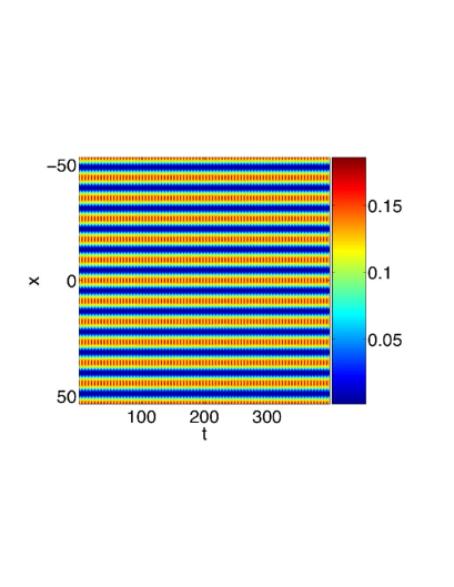
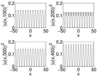
Figure 1: Evolution of the non-resonant spatially extended solution of Eq. (12) with $C$ and $D$ in Eq. (21) given by Eq. (23) [see text for parameter details] for an OSL potential with $V_{2}=2V_{1}=2$ and $\kappa_{2}=3\kappa_{1}=3$. The left panel shows the spatio-temporal evolution of $|u(x,t)|^{2}$ by means of a colored contour plot. The right panel shows spatial profiles of $|u|^{2}$ at four values of time ($t=100$, $200$, $300$, and $400$).

3.2 Resonances

In this subsection, we consider harmonic resonances, additive ultrasubharmonic resonances, and subtractive ultrasubharmonic resonances. In the evolution equations for the slow dynamics, one inserts the appropriate resonance relation into $\Delta$ and $f_{1}$–$f_{7}$. The function $f_{8}$ has both the non-resonant contributions discussed above and additional resonant terms due to the OSL. Note additionally that there is a symmetry-breaking in the resulting equations because the functional form of the lattice contains only cosine terms.

3.2.1 Harmonic Resonances

When $\kappa_{j}=\pm\sqrt{\delta}$, there is a harmonic resonance. The effective equations governing the $O(\varepsilon^{2})$ slow evolution in the presence of a harmonic resonance with respect to the primary lattice wave number $\kappa_{1}$ are

$$C^{\prime} =\frac{1}{\Delta(\kappa_{1},\kappa 2)}\left[\left(f_{1}(\alpha,\kappa_{1},\kappa_{2})B^{2}+f_{2}(\alpha,\kappa_{1},\kappa_{2})A^{2}+f_{3}(\alpha,\kappa_{1},\kappa_{2},b_{1})\right)D+f_{4}(\alpha,\kappa_{1},\kappa_{2})ABC\right.$$

$$\quad\left.+f_{5}(\alpha,\kappa_{1},\kappa_{2})B^{5}+f_{6}(\alpha,\kappa_{1},\kappa_{2})A^{2}B^{3}+f_{7}(\alpha,\kappa_{1},\kappa_{2})A^{4}B+f_{8s}(\alpha,\kappa_{1},\kappa_{2},b_{2})B\right]\,,$$

$$D^{\prime} =\frac{1}{\Delta(\kappa_{1},\kappa 2)}\left[\left(f_{1}(\alpha,\kappa_{1},\kappa_{2})A^{2}+f_{2}(\alpha,\kappa_{1},\kappa_{2})B^{2}+f_{3}(\alpha,\kappa_{1},\kappa_{2},b_{1})\right)C+f_{4}(\alpha,\kappa_{1},\kappa_{2})ABD\right.$$

$$\quad\left.+f_{5}(\alpha,\kappa_{1},\kappa_{2})A^{5}+f_{6}(\alpha,\kappa_{1},\kappa_{2})A^{3}B^{2}+f_{7}(\alpha,\kappa_{1},\kappa_{2})AB^{4}+f_{8c}(\alpha,\kappa_{1},\kappa_{2})A\right]\,,$$ (27)

where

$$\Delta(\kappa_{1},\kappa_{2})=768\kappa_{1}^{3}(4\kappa_{1}^{2}-\kappa_{2}^{2})$$ (28)

and

$$f_{1}(\alpha,\kappa_{1},\kappa_{2}) =3f_{2}(\alpha,\kappa_{1},\kappa_{2})\,,$$

$$f_{2}(\alpha,\kappa_{1},\kappa_{2}) =288\alpha\kappa_{1}^{2}(\kappa_{2}^{2}-4\kappa_{1}^{2})\,,$$

$$f_{3}(\alpha,\kappa_{1},\kappa_{2},b_{1}) =768\kappa_{1}^{4}b_{1}(-\kappa_{2}^{2}+4\kappa_{1}^{2})\,,$$

$$f_{4}(\alpha,\kappa_{1},\kappa_{2}) =2f_{2}(\alpha,\kappa_{1},\kappa_{2})\,,$$

$$f_{5}(\alpha,\kappa_{1},\kappa_{2}) =45\alpha^{2}(-\kappa_{2}^{2}+4\kappa_{1}^{2})\,,$$

$$f_{6}(\alpha,\kappa_{1},\kappa_{2}) =2f_{5}(\alpha,\delta,\kappa_{1},\kappa_{2})\,,$$

$$f_{7}(\alpha,\kappa_{1},\kappa_{2}) =f_{5}(\alpha,\delta,\kappa_{1},\kappa_{2})\,,$$

$$f_{8s}(\alpha,\kappa_{1},\kappa_{2},b_{2}) =f_{non}(\alpha,\kappa_{1},\kappa_{2})+32V_{1}^{2}(\kappa_{2}^{2}-4\kappa_{1}^{2})\,,$$

$$f_{8c}(\alpha,\kappa_{1},\kappa_{2}) =f_{non}(\alpha,\kappa_{1},\kappa_{2})-160V_{1}^{2}(\kappa_{2}^{2}-4\kappa_{1}^{2})\,,$$

$$f_{non}(\alpha,\kappa_{1},\kappa_{2}) =192\kappa_{1}^{2}(V_{2}^{2}-4\kappa_{1}^{2}\kappa_{2}^{2}b_{2}+16\kappa_{1}^{4}b_{2})\,.$$ (29)

If considering a harmonic resonance with respect to the secondary lattice wavenumber $\kappa_{2}$, one obtains the appropriate equations for the $O(\varepsilon^{2})$ slow evolution by switching the roles of $\kappa_{1}$ and $\kappa_{2}$. Note that the form of equations (29) corresponds to (25) except for the extra terms in $f_{8c}$ and $f_{8s}$ that arise from the superlattice.

The equilibria of (27) are given by Eq. (26) except that one inserts the functions from (29). Additionally, the expressions for $C$ and $D$ have $f_{8s}$ rather than $f_{8}$ as a prefactor for $B$ and $f_{8c}$ rather than $f_{8}$ as a prefactor for $A$. One also inserts an equilibrium value of $A$ and $B$ from Eq. (19). One then inserts equilibrium values of $A$, $B$, $C$, and $D$ into Eqs. (15) and (21) to obtain the spatial profile $R=R_{0}+\varepsilon R_{1}+O(\varepsilon^{2})$ to use as an initial condition in direct numerical simulations of Eq. (3).

A typical example of the single-wavelength resonant case is shown in Fig. 2, with $V_{2}=2V_{1}=2$ and $\kappa_{2}=4\kappa_{1}=4\sqrt{\delta}=\pi/b$, where $b$ is the stretching factor of Eq. (11); we used $b_{1}=b_{2}=1$ and $\epsilon=0.1$. The resulting (spatial) quasiperiodic patterns were generically found to persist in the dynamics of the system as stable (temporally oscillating) solutions.

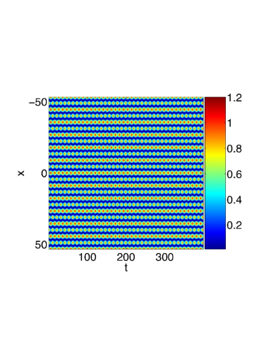
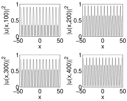
Figure 2: Same as Fig. 1, but for the harmonic resonant case with respect to the primary lattice wavelength. The solution given by Eq. (12) is used as an initial condition with $C$ and $D$ in Eq. (21) given by Eq. (27) with the functions (28, 29) [see text for parameter details].

3.2.2 Ultrasubharmonic Resonances

Studying BECs in an OSL rather than in a regular OL allows one to examine the ultrasubharmonic spatial resonances resulting from interactions between the two lattice wavelengths [44]. As with harmonic resonances, an $O(\varepsilon^{2})$ calculation is required to perform the analysis.

When $\kappa_{2}+\kappa_{1}=\pm 2\sqrt{\delta}$, one has an additive ultrasubharmonic resonance. The effective equations governing the $O(\varepsilon^{2})$ slow evolution in this case are (27) with

$$\Delta(\kappa_{1},\kappa_{2})=32\kappa_{1}\kappa_{2}(\kappa_{1}+2\kappa_{2})(2\kappa_{1}+\kappa_{2})(\kappa_{1}+\kappa_{2})^{3}$$ (30)

and

$$f_{1}(\alpha,\kappa_{1},\kappa_{2}) =3f_{2}(\alpha,\kappa_{1},\kappa_{2})\,,$$

$$f_{2}(\alpha,\kappa_{1},\kappa_{2}) =-24\alpha\kappa_{1}\kappa_{2}[2(\kappa_{1}^{4}+\kappa_{2}^{4})+9(\kappa_{1}^{3}+\kappa_{2}^{3})+14\kappa_{1}^{2}\kappa_{2}^{2}]\,,$$

$$f_{3}(\alpha,\kappa_{1},\kappa_{2},b_{1}) =16\kappa_{1}\kappa_{2}b_{1}[2(\kappa_{1}^{6}+\kappa_{2}^{6})+13\kappa_{1}\kappa_{2}(\kappa_{1}^{4}+\kappa_{2}^{4})+34\kappa_{1}^{2}\kappa_{2}^{2}(\kappa_{1}^{2}+\kappa_{2}^{2})+46\kappa_{1}^{3}\kappa_{2}^{3}]\,,$$

$$f_{4}(\alpha,\kappa_{1},\kappa_{2}) =2f_{2}(\alpha,\kappa_{1},\kappa_{2})\,,$$

$$f_{5}(\alpha,\kappa_{1},\kappa_{2}) =15\alpha^{2}\kappa_{1}\kappa_{2}[5\kappa_{1}\kappa_{2}+2(\kappa_{1}^{2}+\kappa_{2}^{2})]\,,$$

$$f_{6}(\alpha,\kappa_{1},\kappa_{2}) =2f_{5}(\alpha,\delta,\kappa_{1},\kappa_{2})\,,$$

$$f_{7}(\alpha,\kappa_{1},\kappa_{2}) =f_{5}(\alpha,\delta,\kappa_{1},\kappa_{2})\,,$$

$$f_{8s}(\alpha,\kappa_{1},\kappa_{2},b_{2}) =f_{non}(\alpha,\kappa_{1},\kappa_{2})-f_{res}(\alpha,\kappa_{1},\kappa_{2})\,,$$

$$f_{8c}(\alpha,\kappa_{1},\kappa_{2},b_{2}) =f_{non}(\alpha,\kappa_{1},\kappa_{2})+f_{res}(\alpha,\kappa_{1},\kappa_{2})\,,$$

$$f_{non}(\alpha,\kappa_{1},\kappa_{2}) =16[13\kappa_{1}^{2}\kappa_{2}^{2}b_{2}(\kappa_{1}^{4}+\kappa_{2}^{4})+46\kappa_{1}^{4}\kappa_{2}^{4}b_{2}+5\kappa_{1}^{2}\kappa_{2}^{2}(V_{1}^{2}+V_{2}^{2})$$

$$\quad+2\kappa_{1}\kappa_{2}(V_{2}^{2}\kappa_{1}^{2}+V_{1}^{2}\kappa_{2}^{2}+\kappa_{1}^{6}b_{2}+\kappa_{2}^{6}b_{2})+34\kappa_{1}^{3}\kappa_{2}^{3}b_{2}(\kappa_{1}^{2}+\kappa_{2}^{2})$$

$$\quad+4\kappa_{1}\kappa_{2}(V_{1}^{2}\kappa_{1}^{2}+V_{2}^{2}\kappa_{2}^{2})+V_{1}^{2}\kappa_{1}^{4}+V_{2}^{2}\kappa_{2}^{4}]\,,$$

$$f_{res}(\alpha,\kappa_{1},\kappa_{2}) =32V_{1}V_{2}[7\kappa_{1}^{2}\kappa_{2}^{2}+(\kappa_{1}^{4}+\kappa_{2}^{4})+4\kappa_{1}\kappa_{2}(\kappa_{1}^{2}+\kappa_{2}^{2})]\,.$$ (31)

Note that all the terms in $f_{res}$ are proportional to $V_{1}V_{2}$, as they arise from the effects of interacting lattice wavelengths.

Equilibria in this situation again satisfy (26) except that one now inserts functions from (30, 31). Again, the expressions for $C$ and $D$ have $f_{8s}$ rather than $f_{8}$ as a prefactor for $B$ and $f_{8c}$ rather than $f_{8}$ as a prefactor for $A$. One again inserts an equilibrium value of $A$ and $B$ from Eq. (19). One then inserts equilibrium values of $A$, $B$, $C$, and $D$ into Eqs. (15) and (21) to obtain the initial spatial profile $R=R_{0}+\varepsilon R_{1}+O(\varepsilon^{2})$.

A typical simulation of an ultrasubharmonic resonance is shown in Fig. 3, with $V_{2}=2V_{1}=2$ and $\kappa_{2}=3\kappa_{1}=3\sqrt{\delta}/2=3\pi/(8b)$, where $b$ is again given by Eq. (11) with $b_{1}=b_{2}=1$ and $\epsilon=0.1$. The resulting complex patterns were found to persist as stable dynamical structures (with periodic time dynamics).

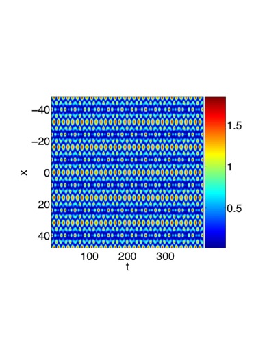
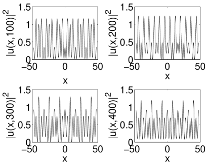
Figure 3: Same as Fig. 1, but for an additive ultrasubharmonic resonance, which arises from the interaction of the BEC’s two wavelengths. The solution of Eq. (12) is used as an initial condition with $C$ and $D$ in Eq. (21) given by Eq. (27) with the functions (30, 31) [see text for parameter details].

When $\kappa_{2}-\kappa_{1}=\pm 2\sqrt{\delta}$, one has a subtractive ultrasubharmonic resonance. The effective equations governing the $O(\varepsilon^{2})$ slow evolution in this case are again (27), with

$$\Delta(\kappa_{1},\kappa_{2})=32\kappa_{1}\kappa_{2}(\kappa_{1}-2\kappa_{2})(2\kappa_{1}-\kappa_{2})(\kappa_{1}-\kappa_{2})^{3}$$ (32)

and

$$f_{1}(\alpha,\kappa_{1},\kappa_{2}) =3f_{2}(\alpha,\kappa_{1},\kappa_{2})\,,$$

$$f_{2}(\alpha,\kappa_{1},\kappa_{2}) =24\alpha\kappa_{1}\kappa_{2}[-2(\kappa_{1}^{4}+\kappa_{2}^{4})+9(\kappa_{1}^{3}+\kappa_{2}^{3})-14\kappa_{1}^{2}\kappa_{2}^{2}]\,,$$

$$f_{3}(\alpha,\kappa_{1},\kappa_{2},b_{1}) =16\kappa_{1}\kappa_{2}b_{1}[2(\kappa_{1}^{6}+\kappa_{2}^{6})-13\kappa_{1}\kappa_{2}(\kappa_{1}^{4}+\kappa_{2}^{4})+34\kappa_{1}^{2}\kappa_{2}^{2}(\kappa_{1}^{2}+\kappa_{2}^{2})-46\kappa_{1}^{3}\kappa_{2}^{3}]\,,$$

$$f_{4}(\alpha,\kappa_{1},\kappa_{2}) =2f_{2}(\alpha,\kappa_{1},\kappa_{2})\,,$$

$$f_{5}(\alpha,\kappa_{1},\kappa_{2}) =15\alpha^{2}\kappa_{1}\kappa_{2}[-5\kappa_{1}\kappa_{2}+2(\kappa_{1}^{2}+\kappa_{2}^{2})]\,,$$

$$f_{6}(\alpha,\kappa_{1},\kappa_{2}) =2f_{5}(\alpha,\delta,\kappa_{1},\kappa_{2})\,,$$

$$f_{7}(\alpha,\kappa_{1},\kappa_{2}) =f_{5}(\alpha,\delta,\kappa_{1},\kappa_{2})\,,$$

$$f_{8s}(\alpha,\kappa_{1},\kappa_{2},b_{2}) =f_{non}(\alpha,\kappa_{1},\kappa_{2})-f_{res}(\alpha,\kappa_{1},\kappa_{2})\,,$$

$$f_{8c}(\alpha,\kappa_{1},\kappa_{2},b_{2}) =f_{non}(\alpha,\kappa_{1},\kappa_{2})+f_{res}(\alpha,\kappa_{1},\kappa_{2})\,,$$

$$f_{non}(\alpha,\kappa_{1},\kappa_{2}) =16[-13\kappa_{1}^{2}\kappa_{2}^{2}b_{2}(\kappa_{1}^{4}+\kappa_{2}^{4})-46\kappa_{1}^{4}\kappa_{2}^{4}b_{2}-5\kappa_{1}^{2}\kappa_{2}^{2}(V_{1}^{2}+V_{2}^{2})$$

$$\quad+2\kappa_{1}\kappa_{2}(V_{2}^{2}\kappa_{1}^{2}+V_{1}^{2}\kappa_{2}^{2}+\kappa_{1}^{6}b_{2}+\kappa_{2}^{6}b_{2})+34\kappa_{1}^{3}\kappa_{2}^{3}b_{2}(\kappa_{1}^{2}+\kappa_{2}^{2})$$

$$\quad+4\kappa_{1}\kappa_{2}(V_{1}^{2}\kappa_{1}^{2}+V_{2}^{2}\kappa_{2}^{2})-V_{1}^{2}\kappa_{1}^{4}-V_{2}^{2}\kappa_{2}^{4}]\,,$$

$$f_{res}(\alpha,\kappa_{1},\kappa_{2}) =32V_{1}V_{2}[-7\kappa_{1}^{2}\kappa_{2}^{2}-(\kappa_{1}^{4}+\kappa_{2}^{4})+4\kappa_{1}\kappa_{2}(\kappa_{1}^{2}+\kappa_{2}^{2})]\,.$$ (33)

As with the additive ultrasubharmonic resonance, all the terms in $f_{res}$ are proportional to $V_{1}V_{2}$.

Equilibria in this case again satisfy (26) except that one inserts the functions from (32, 33). Recall once more that the expressions for $C$ and $D$ have $f_{8s}$ rather than $f_{8}$ as a prefactor for $B$ and $f_{8c}$ rather than $f_{8}$ as a prefactor for $A$. One also inserts an equilibrium value of $A$ and $B$ from Eq. (19). One then inserts equilibrium values of $A$, $B$, $C$, and $D$ into Eqs. (15) and (21) to obtain a spatial profile $R=R_{0}+\varepsilon R_{1}+O(\varepsilon^{2})$ to utilize as an initial wavefunction in numerical simulations of (3). In this case, the numerical simulations yielded similar (stable) temporal dynamics as for additive ultrasubharmonic resonances.

4 Hamiltonian Perturbation Theory and Subharmonic Resonances

In this section, we build on recent work [49, 50] and apply Hamiltonian perturbation theory to (10) to examine period-multiplied wavefunctions and spatial subharmonic resonances in repulsive BECs loaded into OSL potentials. (For expository reasons, we repeat some details of the derivation from those works in the present one.) We perturb off elliptic function solutions of the underlying integrable system and study $2n\!:\!1$ spatial resonances with a leading-order perturbation method. Perturbing off simple harmonic functions, by contrast, requires a perturbative method of order $n$ to study $2n\!:\!1$ resonances. At the center of KAM islands lie ‘period-multiplied’ states. When $n=1$, one obtains period-doubled states in $u$ corresponding to $2\!:\!1$ subharmonic resonances. Our analysis reveals period-multiplied solutions of the GP (3) with respect to both the primary and secondary sublattice.

The dynamical systems perspective on period-doubled states and their generalizations for BECs in OSL potentials given here complements theoretical and experimental work by other authors for the case of regular OL potentials. In recent experiments, Gemelke et al. [26] constructed period-doubled wavefunctions, which have received increased attention (for regular lattices) during the past two years. In earlier work, Smerzi et al. [56] reported theoretical studies of spatial period-doubling in the context of modulational (“dynamical”) instabilities of Bloch states and Cataliotti et al. [19] reported experimental observations of superfluid current disruption in chains of weakly coupled BECs. Period-doubled states, interpreted as soliton trains, then arise from dynamical instabilities of the energy bands associated with Bloch states [39].

4.1 Unforced Duffing Oscillator

We employ exact elliptic function solutions of Duffing’s equation [Eq. (10) with $V_{1}=V_{2}=0$], so we no longer need to assume the coefficient of the nonlinearity is small. Therefore, we use the ODE

$$R^{\prime\prime}+\delta R+\alpha R^{3}+\varepsilon R[V_{1}\cos(\kappa_{1}x)+V_{2}\cos(\kappa_{2}x)]=0\,,$$ (34)

which is just like (10) except that $\alpha$ no longer has the prefactor $\varepsilon$.

When $\varepsilon=0$, solutions of (34) are expressed exactly in terms of elliptic functions (see, e.g., [62, 50] and references therein):

$$R=\sigma\rho\,\mbox{cn}(u,k)\,,$$ (35)

where

$$u =u_{1}x+u_{0}\,,\quad u_{1}^{2}=\delta+\alpha\rho^{2}\,,$$

$$k^{2} =\frac{\alpha\rho^{2}}{2(\delta+\alpha\rho^{2})}\,,$$

$$u_{1} \geq 0,\hskip 7.22743pt\rho\geq 0\,,\hskip 7.22743ptk^{2}\in\mathbb{R}\,,\hskip 7.22743pt\sigma\in\{-1,1\}\,,$$ (36)

and $u_{0}$ is obtained from an initial condition (and can be set to $0$ without loss of generality). When $u_{1}\in\mathbb{R}$, the solutions given by (36) are periodic. When $k^{2}<0$, which is the case for repulsive BECs with positive chemical potentials, equation (36) is interpreted using the reciprocal complementary modulus transformation (as discussed in Ref. [50]).

Equation (34) is integrated when $\varepsilon=0$ to yield the Hamiltonian

$$\frac{1}{2}R^{\prime 2}+\frac{1}{2}\delta R^{2}+\frac{1}{4}\alpha R^{4}=h\,,$$ (37)

with given energy

$$h=\frac{1}{4}\rho^{2}(2\delta+\alpha\rho^{2})=\frac{\delta^{2}}{\alpha}\frac{k^{2}k^{\prime 2}}{(1-2k^{2})^{2}}\,,$$ (38)

where $k^{\prime 2}:=1-k^{2}$.

The center at $(0,0)$ satisfies $h=\rho^{2}=k^{2}=0$. The saddles at $(\pm\sqrt{-\delta/\alpha},0)$ and their adjoining separatrix (consisting of two heteroclinic orbits) satisfy

$$h=-\frac{\delta^{2}}{4\alpha}\,,\quad\rho^{2}=\frac{\delta}{|\alpha|}\,,\quad k^{2}=-\infty\,.$$ (39)

The sign $\sigma=+1$ is used for the right saddle and $\sigma=-1$ is used for the left one. Within the separatrix, all orbits are periodic and the value of $\sigma$ is immaterial.

4.2 Action-Angle Variable Description and Transformations

For the sake of exposition, we construct an action-angle description in steps. First, we rescale (34) using the coordinate transformation

$$\chi=\sqrt{\delta}x\,,\qquad r=\sqrt{-\frac{\alpha}{\delta}}R$$ (40)

to obtain

$$r^{\prime\prime}+r-r^{3}=0$$ (41)

when $V_{1}=V_{2}=0$. In terms of the original coordinates,

$$R(x)=\sqrt{-\frac{\delta}{\alpha}}r\left(\sqrt{\delta}x\right)\,.$$ (42)

The Hamiltonian corresponding to (41) is

$$H_{0}(r,s)=\frac{1}{2}s^{2}+\frac{1}{2}r^{2}-\frac{1}{4}r^{4}=h\,,\quad h\in[0,1/4]\,,$$ (43)

where $s:=r^{\prime}=dr/d\chi$. Additionally, $\rho^{2}\in[0,1]$ and

$$k^{2}=\frac{\rho^{2}}{2(\rho^{2}-1)}\,.$$ (44)

With the initial condition $r(0)=\rho$, $s(0)=0$ (which implies that $u_{0}=0$), solutions to (41) are given by

$$r(\chi) =\rho\,\mbox{cn}\left(\left[1-\rho^{2}\right]^{1/2}\chi,k\right)\,,$$

$$s(\chi) =-\rho\left[1-\rho^{2}\right]^{1/2}\,\mbox{sn}\left(\left[1-\rho^{2}\right]^{1/2}\chi,k\right)\mbox{dn}\left(\left[1-\rho^{2}\right]^{1/2}\chi,k\right)\,.$$ (45)

The period of a given periodic orbit $\Gamma$ is

$$T(k)=\oint_{\Gamma}d\chi=\frac{4K(k)}{\sqrt{1-\rho^{2}}}\,,$$ (46)

where $4K(k)$ is the period in $u$ of $\mbox{cn}(u,k)$ [59]. The frequency of this orbit is

$$\Omega(k)=\frac{\pi\sqrt{1-\rho^{2}}}{2K(k)}\,.$$ (47)

Let $\Gamma_{h}$ denote the periodic orbit with energy $h=H_{0}(r,s)$. The area of phase space enclosed by this orbit is constant with respect to $\chi$, so we define the action [27]

$$J:=\frac{1}{2\pi}\oint_{\Gamma_{h}}sdr=\frac{1}{2\pi}\int_{0}^{T(k)}[s(\chi)]^{2}d\chi\,,$$ (48)

which is evaluated to obtain

$$J=\frac{4\sqrt{1-\rho^{2}}}{3\pi}\left[E(k)-\left(1-\rho^{2}/2\right)K(k)\right]\,.$$ (49)

The associated angle in the canonical transformation $(r,s)\longrightarrow(J,\Phi)$ is

$$\Phi:=\Phi(0)+\Omega(k)\chi\,.$$ (50)

The frequency $\Omega(k)$ decreases monotonically as $k^{2}$ goes from $-\infty$ to $0$ [that is, as one goes from the separatrix to the center at $(r,s)=(0,0)$]. With this transformation, equation (45) becomes

$$r(J,\Phi) =\rho(J)\,\mbox{cn}\left(2K(k)\Phi/\pi,k\right)\,,$$

$$s(\chi) =-\rho(J)\sqrt{1-\rho(J)^{2}}\,\mbox{sn}\left(2K(k)\Phi/\pi,k\right)\mbox{dn}\left(2K(k)\Phi/\pi,k\right)\,,$$ (51)

where $k=k(J)$.

After rescaling, the equations of motion for the forced system (34) take the form

$$r^{\prime\prime}+r-r^{3}+\frac{\varepsilon}{\delta}\left[V_{1}\cos\left(\frac{\kappa_{1}}{\sqrt{\delta}}\chi\right)+V_{2}\cos\left(\frac{\kappa_{2}}{\sqrt{\delta}}\chi\right)\right]r=0$$ (52)

with the corresponding Hamiltonian

$$H(r,s,\chi) =H_{0}(r,s)+\varepsilon H_{1}(r,s,\chi)$$

$$=\frac{1}{2}s^{2}+\frac{1}{2}r^{2}-\frac{1}{4}r^{4}+\frac{\varepsilon}{2\delta}r^{2}\left[V_{1}\cos\left(\frac{\kappa_{1}}{\sqrt{\delta}}\chi\right)+V_{2}\cos\left(\frac{\kappa_{2}}{\sqrt{\delta}}\chi\right)\right]\,.$$ (53)

In action-angle coordinates, this becomes

$$H(\Phi,J,\chi)=\frac{1}{2}\rho(J)^{2}-\frac{1}{4}\rho(J)^{4}+\frac{\varepsilon}{2\delta}\rho(J)^{2}\,\mbox{cn}^{2}\left(2K(k)\Phi/\pi,k\right)\left[V_{1}\cos\left(\frac{\kappa_{1}}{\sqrt{\delta}}\chi\right)+V_{2}\cos\left(\frac{\kappa_{2}}{\sqrt{\delta}}\chi\right)\right]\,.$$ (54)

A more convenient action-angle pair $(\phi,j)$ is obtained using the canonical transformation $(\Phi,J)\longrightarrow(\phi,j)$, defined by the relations

$$j(J)=\frac{1}{2}\rho(J)^{2}\,,\quad\Phi(\phi,j)=\frac{\phi}{J^{\prime}(j)}\,,$$ (55)

where

$$k^{2} =\frac{j}{2j-1}\,,$$

$$J(j) =\frac{2}{3}\sqrt{1-2j}\left[\tilde{E}(j)-(1-j)\tilde{K}(j)\right]\,,$$

$$\tilde{K}(j) =\frac{2}{\pi}K[k(j)]\,,\quad\tilde{E}(j)=\frac{2}{\pi}E[k(j)]\,.$$ (56)

Additionally,

$$J^{\prime}(j):=\frac{dJ}{dj}=\sqrt{1-2j}\tilde{K}(j)=\frac{1-2j}{\Omega(j)}\,.$$ (57)

Note that $J\sim j$ for small-amplitude motion. Furthermore, $j=0$ at the origin, and $j=1/2$ on the separatrix. The Hamiltonian (54) becomes

$$H(\phi,j,\chi)=j-j^{2}+\frac{\epsilon}{\delta}j\,\mbox{cn}^{2}\left(\frac{\tilde{K}(j)}{J^{\prime}(j)}\phi,k\right)\left[V_{1}\cos\left(\frac{\kappa_{1}}{\sqrt{\delta}}\chi\right)+V_{2}\cos\left(\frac{\kappa_{2}}{\sqrt{\delta}}\chi\right)\right]\,.$$ (58)

4.3 Perturbative Analysis

A subsequent $\mathcal{O}(\epsilon)$ analysis at this stage allows us to study $2n\!:\!1$ subharmonic resonances for all $n\in\mathbb{Z}$. Fourier expanding the cn function yields

$$\mbox{cn}^{2}\left(\frac{\tilde{K}(j)}{J^{\prime}(j)}\phi,k\right)=\mathcal{B}_{0}(j)+\sum_{l=1}^{\infty}\mathcal{B}_{l}\cos\left(\frac{2l\phi}{J^{\prime}(j)}\right)\,,$$ (59)

where the coefficients $\mathcal{B}_{l}(j)$ are obtained by convolving the Fourier coefficients [62, 50],

$$B_{n}(j) =\frac{4}{k(j)\tilde{K}(j)}b_{n}[k(j)]\,,$$

$$b_{n}(k) =\frac{1}{2}\mbox{sech}\left[\left(n+1/2\right)\pi K^{\prime}(k)/K(k)\right]\,,$$ (60)

of the cn function in Eq. (58), where $K^{\prime}(k):=K(\sqrt{1-k^{2}})$ is the complementary complete elliptic integral of the first kind [59, 1].

The resulting $O(\varepsilon)$ term in the Hamiltonian (58) is

$$\varepsilon H_{1}(\phi,j,\chi) =\frac{\varepsilon}{\delta}j\mathcal{B}_{0}(j)\left[V_{1}\cos\left(\frac{\kappa_{1}}{\sqrt{\delta}}\chi\right)+V_{2}\cos\left(\frac{\kappa_{2}}{\sqrt{\delta}}\chi\right)\right]$$

$$\quad+\frac{\varepsilon}{2\delta}jV_{1}\sum_{l=1}^{\infty}\mathcal{B}_{l}(j)\left[\cos\left(\frac{2l\phi}{J^{\prime}(j)}+\frac{\kappa_{1}}{\sqrt{\delta}}\chi\right)+\cos\left(\frac{2l\phi}{J^{\prime}(j)}-\frac{\kappa_{1}}{\sqrt{\delta}}\chi\right)\right]$$

$$\quad+\frac{\varepsilon}{2\delta}jV_{2}\sum_{l^{\prime}=1}^{\infty}\mathcal{B}_{l^{\prime}}(j)\left[\cos\left(\frac{2l^{\prime}\phi}{J^{\prime}(j)}+\frac{\kappa_{2}}{\sqrt{\delta}}\chi\right)+\cos\left(\frac{2l^{\prime}\phi}{J^{\prime}(j)}-\frac{\kappa_{2}}{\sqrt{\delta}}\chi\right)\right]\,.$$ (61)

The Hamiltonian (61) is an expansion over infinitely many subharmonic resonance bands for each of the primary and secondary lattice wavenumbers. Each resonance corresponds to a single harmonic in (61). To isolate individual resonances, we apply the canonical, near-identity transformation [62, 50]

$$\phi =Q_{i}+\varepsilon\frac{\partial W_{1}}{\partial P}+\mathcal{O}(\varepsilon^{2})\,,$$

$$j =P-\varepsilon\frac{\partial W_{1}}{\partial Q_{i}}+\mathcal{O}(\varepsilon^{2})$$ (62)

to (61) with an appropriate generating function $W_{1}$ that removes all the resonances except the one of interest. The subscript $i$ in $Q_{i}$ designates whether one is considering a resonance with respect to the primary or secondary lattice wavenumber. The transformation (62) is valid in a neighborhood of this $2n\!:\!1$ resonance and yields an autonomous 1 DOF resonance Hamiltonian that determines its local dynamics,

$$K(Q,P,\chi;n) =P-P^{2}+\frac{\varepsilon}{2\delta}V_{i}P\mathcal{B}_{n}(P)\cos\left(\frac{2nQ_{i}}{J^{\prime}(P)}-\frac{\kappa_{i}}{\sqrt{\delta}}\chi\right)+\mathcal{O}(\epsilon^{2})\,.$$ (63)

In focusing on a single resonance band in phase space, one restricts $P$ to a neighborhood of $P_{n}$, which denotes the location of the $n$th resonant torus associated with periodic orbits in $2n\!:\!1$ spatial resonance with the primary ($i=1$) or secondary ($i=2$) sublattice (recall that $\kappa_{1}<\kappa_{2}$).

The resonance relation associated with $2n\!:\!1$ resonances with respect to the $i$th sublattice is [50]

$$\frac{\kappa_{i}}{\sqrt{\delta}}=\pm 2n\Omega(P_{n})\,.$$ (64)

Because $\Omega\leq 1$ is a decreasing function of $P\in[0,1/2)$, the associated resonance band is present when

$$\frac{\kappa_{i}}{\sqrt{\delta}}\leq 2n\,.$$ (65)

For example, when $\kappa_{i}=2.5$ and $\delta=1$, there are resonances of order $4\!:\!1$, $6\!:\!1$, $8\!:\!1$, etc, but there are no resonances or order $2\!:\!1$. Analytical expressions for the sizes of the resonance bands and the locations of their saddles and centers are the same as those obtained for BECs loaded into OLs; they are derived in Ref. [50].

To examine the time-evolution of period-multiplied solutions, we need only the locations of centers, which are obtained by applying one more canonical transformation. We use the generating function

$$F_{i}(Q_{i},Y,\chi;n)=Q_{i}Y-\frac{\kappa_{i}}{2n\sqrt{\delta}}J(Y)\chi\,,$$ (66)

which yields

$$P =\frac{\partial F_{i}}{\partial Q_{i}}(Q_{i},Y,\chi)=Y\,,$$

$$\xi =\frac{\partial F_{i}}{\partial Y}(Q_{i},Y,\chi)=Q_{i}-\frac{\kappa_{i}}{2n\sqrt{\delta}}J^{\prime}(Y)\chi\,.$$ (67)

The resonance Hamiltonian (63) becomes

$$K_{n}(\xi,Y) =K(Q_{i},P,\chi;n)+\frac{\partial F_{i}}{\partial\chi}(Q_{i},Y,\chi)$$

$$=Y-Y^{2}-\frac{\kappa_{i}}{2n\sqrt{\delta}}J(Y)+\frac{\varepsilon}{2\delta}V_{i}Y\mathcal{B}_{n}(Y)\cos\left(\frac{2n\xi}{J^{\prime}(Y)}\right)\,,$$ (68)

which is integrable in the $(Y,\xi)$ coordinate system.

The centers of the KAM islands associated with this resonance occur at [50]

$$Y_{c}=Y_{n}+\varepsilon\Delta Y+\mathcal{O}(\varepsilon^{2})\,,$$ (69)

where

$$\Delta Y=\mp\frac{1}{2\delta}\left[\frac{\mathcal{B}_{n}(Y_{n})+Y_{n}\mathcal{B}_{n}^{\prime}(Y_{n})}{\Omega(Y_{n})\sqrt{1-2Y_{n}}\tilde{K}^{\prime}(Y_{n})-1}\right]\,,$$ (70)

and the sign is $-$ when $n$ is even and $+$ when $n$ is odd. One then converts the value $Y_{c}$ back to the original coordinates to obtain an estimate $(R_{c},S_{c})$ of the location of the center in phase space. [One obtains the locations of the other centers associated with the same resonance band using iterates of $(R_{c},S_{c})$ under a Poincaré map, but we only need one of these centers for a given resonance to examine the time-evolution under the GP equation (3) of these solutions, which provide the initial wavefunctions for the PDE simulations.]

In our numerical computations, we use the parameter values $\hbar=2m=1$, $\delta=1$, $\alpha=-1$, $\varepsilon=0.01$, and $V_{1}=1$ in Eqs. (3, 34). With $\kappa=1.5$, there is a center for the $2\!:\!1$ resonance with respect to the primary sublattice at $R_{c}\approx 0.753$ and $S_{c}=0$, so one uses $R=0.753\cos(\kappa_{1}x/2)$ as an initial wavefunction in simulations of (3) for any height $V_{2}$ and wavenumber $\kappa_{2}$ of the secondary sublattice. Such a solution is shown in Fig. 4 for $V_{2}=2$ and $\kappa_{2}=3\kappa_{1}$. It is dynamically stable and sustains only small amplitude variations (but is otherwise essentially stationary). One can similarly examine initial wavefunctions corresponding to $2\!:\!1$ resonances with respect to the secondary sublattice.

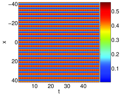
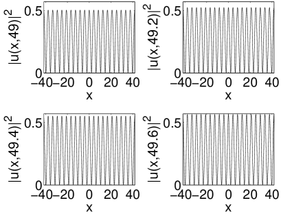
Figure 4: Same as Fig. 1, but for a $2\!:\!1$ resonance with respect to the primary sublattice. The solution described in the text [$R=0.753\cos(\kappa_{1}x/2)$ with $\kappa_{1}=1.5=\kappa_{2}/3$] is used as the initial condition (see the text for further parameter details). The solution appears to be dynamically stable and only sustains a small-amplitude oscillation.

With $\kappa_{1}=2.5$, there is a center for the $4\!:\!1$ resonance with respect to the primary sublattice at $(R_{c},S_{c})\approx(0.691,0.324)$, so (recalling the chain rule) one uses $R=0.691\cos(\kappa_{1}x/4)+0.518\sin(\kappa_{1}x/4)$ as an initial wavefunction in simulations of (3) The results with $\kappa_{2}=3\kappa_{1}$ and $V_{2}=2$ are shown in Fig. 5. We observe a wriggling pattern in the contour plot (in the left panel), which indicates (structurally stable) spatio-temporally oscillatory behavior of the condensate.

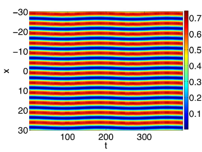
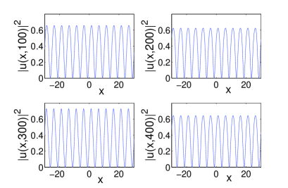
Figure 5: Same as Fig. 1, but for a $4\!:\!1$ resonance with respect to the primary sublattice. The solution described in the text [$R=0.691\cos(\kappa_{1}x/4)+0.518\sin(\kappa_{1}x/4)$ with $\kappa_{1}=2.5=\kappa_{2}/3$] is used as the initial condition (see the text for further parameter details). While structurally stable, the solution pattern appears to be a wriggling one, indicating a spatio-temporal breathing.

With $\kappa_{1}=3.8$, there is a center for the $6\!:\!1$ resonance with respect to the primary sublattice at $R_{c}\approx 0.859$ and $S_{c}=0$, so one uses $R=0.859\cos(\kappa_{1}x/6)$ as an initial wavefunction in simulations of (3). We observe that this period-multiplied state is stable with small-amplitude oscillations, as was the case for $2\!:\!1$ resonances. At the same value of $\kappa_{1}$, there is a center for the $8\!:\!1$ resonance with respect to the primary sublattice at $R_{c}\approx 0.9354$ and $S_{c}\approx 0.0718$, so one uses $R=0.9354\cos(\kappa_{1}x/8)+0.151\sin(\kappa_{1}x/8)$ as an initial wavefunction. As was the case for $4\!:\!1$ resonances, PDE simulations reveal structurally stable spatio-temporally oscillatory behavior of the condensate (shown for $4\!:\!1$ resonances as a wriggling pattern in the left panel of Fig. 5). This difference between “odd” and “even” subharmonic resonances arises from the fact that the former contain centers on the $R$-axis, whereas the latter do not. The resulting initial conditions in the even case hence require both sine and cosine harmonics, resulting in the observed spatio-temporal breathing.

From a more general standpoint, resonance bands emerge from resonant KAM tori at action values $P_{*}$ that satisfy a (three-term) resonance relation with respect to both sublattices [60, 61],

$$n_{1}\frac{\kappa_{1}}{\sqrt{\delta}}+n_{2}\frac{\kappa_{2}}{\sqrt{\delta}}=2n\Omega(P_{*})\,,$$ (71)

where $n$, $n_{1}$, and $n_{2}$ all take integer values. The single-sublattice resonance relation (64) is a special case of (71).

5 Conclusions

In this work, we analyzed spatially extended coherent structure solutions of the Gross-Pitaevskii (GP) equation in optical superlattices describing the dynamics of cigar-shaped Bose-Einstein condensates (BECs) in such potentials. To do this, we derived amplitude equations governing the evolution of spatially modulated states of the BEC. We used second-order multiple scale perturbation theory to study spatial harmonic resonances with respect to a single lattice wavenumber, as well as additive and subtractive ultrasubharmonic resonances. Harmonic resonances are a second-order effect that can occur in regular periodic lattices, but ultrasubharmonic resonances can only occur in superlattice potentials, as they arise from the interaction of multiple lattice wavelengths. In each situation, we determined the resulting dynamical equilibria, which represent spatially periodic solutions, and examined the stability of the corresponding solutions via direct simulations of the GP equation. In every case considered, the solutions (non-resonant, resonant with a single wavelength, and resonant due to interactions between two wavelengths) were found numerically to be dynamically stable under time-evolution of the GP equation. Finally, we used Hamiltonian perturbation theory to construct subharmonically resonant solutions, whose spatio-temporal dynamics we illustrated numerically in a number of prototypical cases.

References

• [1] M. Abramowitz and I. Stegun, eds., Handbook of Mathematical Functions with Formulas, Graphs, and Mathematical Tables, no. 55 in Applied Mathematics Series, National Bureau of Standards, Washington, D. C., 1964.
• [2] G. L. Alfimov, P. G. Kevrekidis, V. V. Konotop, and M. Salerno, Wannier functions analysis of the nonlinear Schrödinger equation with a periodic potential, Physical Review E, 66 (2002), no. 046608.
• [3] B. P. Anderson and M. A. Kasevich, Macroscopic quantum interference from atomic tunnel arrays, Science, 282 (1998), pp. 1686–1689.
• [4] M. H. Anderson, J. R. Ensher, M. R. Matthews, C. E. Wieman, and E. A. Cornell, Observation of Bose-Einstein condensation in a dilute atomic vapor, Science, 269 (1995), pp. 198–201.
• [5] T. Anker, M. Albiez, R. Gati, S. Hunsmann, B. Eiermann, A. Trombettoni, and M. K. Oberthaler, Nonlinear self-trapping of matter waves in periodic potentials, Physical Review Letters, 94 (2005), no. 020403.
• [6] N. W. Ashcroft and N. D. Mermin, Solid State Physics, Brooks/Cole, Australia, 1976.
• [7] B. B. Baizakov, V. V. Konotop, and M. Salerno, Regular spatial structures in arrays of Bose-Einstein condensates induced by modulational instability, Journal of Physics B: Atomic Molecular and Optical Physics, 35 (2002), pp. 5105–5119.
• [8] Y. B. Band, I. Towers, and B. A. Malomed, Unified semiclassical approximation for Bose-Einstein condensates: Application to a BEC in an optical potential, Physical Review A, 67 (2003), no. 023602.
• [9] C. M. Bender and S. A. Orszag, Advanced Mathematical Methods for Scientists and Engineers, McGraw-Hill, New York, NY, 1978.
• [10] K. Berg-Sørensen and K. Mølmer, Bose-Einstein condensates in spatially periodic potentials, Physical Review A, 58 (1998), pp. 1480–1484.
• [11] V. A. Brazhnyi and V. V. Konotop, Theory of nonlinear matter waves in optical lattices, Modern Physics Letters B, 18 (2004), pp. 627-651.
• [12] J. C. Bronski, L. D. Carr, R. Carretero-González, B. Deconinck, J. N. Kutz, and K. Promislow, Stability of attractive Bose-Einstein condensates in a periodic potential, Physical Review E, 64 (2001), no. 056615.
• [13] J. C. Bronski, L. D. Carr, B. Deconinck, and J. N. Kutz, Bose-Einstein condensates in standing waves: The cubic nonlinear Schrödinger equation with a periodic potential, Physical Review Letters, 86 (2001), pp. 1402–1405.
• [14] J. C. Bronski, L. D. Carr, B. Deconinck, J. N. Kutz, and K. Promislow, Stability of repulsive Bose-Einstein condensates in a periodic potential, Physical Review E, 63 (2001), no. 036612.
• [15] L. Brusch, A. Torcini, M. van Hecke, M. G. Zimmermann, and M. Bär, Modulated amplitude waves and defect formation in the one-dimensional complex Ginzburg-Landau equation, Physica D, 160 (2001), pp. 127–148.
• [16] L. Brusch, M. G. Zimmermann, M. van Hecke, M. Bär, and A. Torcini, Modulated amplitude waves and the transition from phase to defect chaos, Physical Review Letters, 85 (2000), pp. 86–89.
• [17] K. Burnett, M. Edwards, and C. W. Clark, The theory of Bose-Einstein condensation of dilute gases, Physics Today, 52 (1999), pp. 37–42.
• [18] R. Carretero-González and K. Promislow, Localized breathing oscillations of Bose-Einstein condensates in periodic traps, Physical Review A, 66 (2002), no. 033610.
• [19] F. S. Cataliotti, L. Fallani, F. Ferlaino, C. Fort, P. Maddaloni, and M. Inguscio, Superfluid current disruption in a chain of weakly coupled Bose-Einstein condensates, New Journal of Physics, 5 (2003), pp. 71.1–71.7.
• [20] D.-I. Choi and Q. Niu, Bose-Einstein condensates in an optical lattice, Physical Review Letters, 82 (1999), pp. 2022–2025.
• [21] F. Dalfovo, S. Giorgini, L. P. Pitaevskii, and S. Stringari, Theory of Bose-Einstein condensation on trapped gases, Reviews of Modern Physics, 71 (1999), pp. 463–512.
• [22] K. B. Davis, M.-O. Mewes, M. R. Andrews, N. J. van Druten, D. S. Durfee, D. M. Kurn, and W. Ketterle, Bose-Einstein condensation in a gas of sodium atoms, Physical Review Letters, 75 (1995), pp. 3969–3973.
• [23] L. A. Dmitrieva and Y. A. Kuperin, Spectral modelling of quantum superlattice and application to the Mott-Peierls simulated transitions. arXiv:cond-mat/0311468, November 19 2003.
• [24] E. A. Donley, N. R. Claussen, S. L. Cornish, J. L. Roberts, E. A. Cornell, and C. E. Weiman, Dynamics of collapsing and exploding Bose-Einstein condensates, Nature, 412 (2001), pp. 295–299.
• [25] Y. Eksioglu, P. Vignolo, and M. P. Tosi, Matter-wave interferometry in periodic and quasi-periodic arrays. arXiv:cond-mat/0404458, April 2004.
• [26] N. Gemelke, E. Sarajlic, Y. Bidel, S. Hong, and S. Chu, Period-doubling instability of Bose-Einstein condensates induced in periodically translated optical lattices. cond-mat/0504311, April 2005.
• [27] H. Goldstein, Classical Mechanics, Addison-Wesley Publishing Company, Reading, MA, 2nd ed., 1980.
• [28] M. Greiner, O. Mandel, T. Esslinger, T. Hänsch, and I. Bloch, Quantum phase transition from a superfluid to a Mott insulator in a gas of ultracold atoms, Nature, 415 (2002), pp. 39–44.
• [29] E. W. Hagley, L. Deng, M. Kozuma, J. Wen, K. Helmerson, S. L. Rolston, and W. D. Phillips, A well-collimated quasi-continuous atom laser, Science, 283 (1999), pp. 1706–1709.
• [30] W. Ketterle, Experimental studies of Bose-Einstein condensates, Physics Today, 52 (1999), pp. 30–35.
• [31] P. G. Kevrekidis, R. Carretero-González, D. J. Frantzeskakis, and I. Kevrekidis, Vortices in Bose-Einstein condensates: Some recent developments, Modern Physics Letters B, 18 (2004), pp. 1481-1505.
• [32] P. G. Kevrekidis and D. J. Frantzeskakis, Pattern forming dynamical instabilities of Bose-Einstein condensates, Modern Physics Letters B, 18 (2004), pp. 173–202.
• [33] P. G. Kevrekidis, D. J. Frantzeskakis, B. A. Malomed, A. R. Bishop, and I. G. Kevrekidis, Dark-in-bright solitons in Bose-Einstein condensates with attractive interactions, New Journal of Physics, 5 (2003), pp. 64.1–64.17.
• [34] P. G. Kevrekidis, G. Theocharis, D. J. Frantzeskakis, and B. A. Malomed, Feshbach resonance management for Bose-Einstein condensates, Physical Review Letters, 90 (2003), no. 230401.
• [35] T. Köhler, Three-body problem in a dilute Bose-Einstein condensate, Physical Review Letters, 89 (2002), no. 210404.
• [36] D. F. Lawden, Elliptic Functions and Applications, no. 80 in Applied Mathematical Sciences, Springer-Verlag, New York, NY, 1989.
• [37] P. J. Y. Louis, E. A. Ostrovskaya, and Y. S. Kivshar, Matter-wave dark solitons in optical lattices, Journal of Optics B: Quantum and Semiclassical Optics, 6 (2004), pp. S309–S317.
• [38] P. J. Y. Louis, E. A. Ostrovskaya, C. M. Savage, and Y. S. Kivshar, Bose-Einstein condensates in optical lattices: Band-gap structure and solitons, Physical Review A, 67 (2003), no. 013602.
• [39] M. Machholm, A. Nicolin, C. J. Pethick, and H. Smith, Spatial period-doubling in Bose-Einstein condensates in an optical lattice, Physical Review A, 69 (2004), no. 043604.
• [40] M. Machholm, C. J. Pethick, and H. Smith, Band structure, elementary excitations, and stability of a Bose-Einstein condensate in a periodic potential, Physical Review A, 67 (2003), no. 053613.
• [41] B. A. Malomed, Z. H. Wang, P. L. Chu, and G. D. Peng, Multichannel switchable system for spatial solitons, Journal of the Optical Society of America B, 16 (1999), pp. 1197–1203.
• [42] O. Morsch, J. H. Müller, M. Christiani, D. Ciampini, and E. Arimondo, Bloch oscillations and mean-field effects of Bose-Einstein condensates in 1D optical lattices, Physical Review Letters, 87 (2001), no. 140402.
• [43] E. J. Mueller, Superfluidity and mean-field energy loops; hysteretic behavior in Bose-Einstein condensates, Physical Review A, 66 (2002), no. 063603.
• [44] A. H. Nayfeh and D. T. Mook, Nonlinear Oscillations, John Wiley & Sons, Inc., New York, NY, 1995.
• [45] C. Orzel, A. K. Tuchman, M. L. Fenselau, M. Yasuda, and M. A. Kasevich, Squeezed states in a Bose-Einstein condensate, Science, 291 (2001), p. 2386.
• [46] P. Pedri, L. Pitaevskii, S. Stringari, C. Fort, S. Burger, F. S. Cataliotii, P. Maddaloni, F. Minardi, and M. Inguscio, Expansion of a coherent array of Bose-Einstein condensates, Physical Review Letters, 87 (2001), no. 220401.
• [47] S. Peil, J. V. Porto, B. Laburthe Tolra, J. M. Obrecht, B. E. King, M. Subbotin, S. L. Rolston, and W. D. Phillips, Patterned loading of a Bose-Einstein condensate into an optical lattice, Physical Review A, 67 (2003), no. 051603(R).
• [48] C. J. Pethick and H. Smith, Bose-Einstein Condensation in Dilute Gases, Cambridge University Press, Cambridge, United Kingdom, 2002.
• [49] M. A. Porter and P. Cvitanović, Modulated amplitude waves in Bose-Einstein condensates, Physical Review E, 69 (2004), no. 047201.
• [50]  , A perturbative analysis of modulated amplitude waves in Bose-Einstein condensates, Chaos, 14 (2004), pp. 739–755.
• [51] M. A. Porter, P. G. Kevrekidis, and B. A. Malomed, Resonant and non-resonant modulated amplitude waves for binary Bose-Einstein condensates in optical lattices, Physica D, 196 (2004), pp. 106–123.
• [52] J. V. Porto, S. Rolston, B. Laburthe Tolra, C. J. Williams, and W. D. Phillips, Quantum information with neutral atoms as qubits, Philosophical Transactions: Mathematical, Physical & Engineering Sciences, 361 (2003), pp. 1417–1427.
• [53] R. H. Rand, Lecture Notes on Nonlinear Vibrations. A free online book available at http://www.tam.cornell.edu/randdocs/nlvibe45.pdf, 2003.
• [54] A. M. Rey, B. L. Hu, E. Calzetta, A. Roura, and C. Clark, Nonequilibrium dynamics of optical lattice-loaded BEC atoms: Beyond HFB approximation, Physical Review A, 69 (2004), no. 033610.
• [55] L. Salasnich, A. Parola, and L. Reatto, Periodic quantum tunnelling and parametric resonance with cigar-shaped Bose-Einstein condensates, Journal of Physics B: Atomic Molecular and Optical Physics, 35 (2002), pp. 3205–3216.
• [56] A. Smerzi, A. Trombettoni, P. G. Kevrekidis, and A. R. Bishop, Dynamical superfluid-insulator transition in a chain of weakly coupled Bose-Einstein condensates, Physical Review Letters, 89 (2002), no. 170402.
• [57] S. Stringari and L. Pitaevskii, Bose-Einstein Condensation, Oxford University Press, Oxford, United Kingdom, 2003.
• [58] K. G. H. Vollbrecht, E. Solano, and J. L. Cirac, Ensemble quantum computation with atoms in periodic potentials, Physical Review Letters, 93 (2004), no. 220502.
• [59] E. T. Whittaker and G. N. Watson, A Course of Modern Analysis, Cambridge University Press, Cambridge, Great Britain, fourth ed., 1927.
• [60] R. S. Zounes and R. H. Rand, Global behavior of a nonlinear quasiperiodic Mathieu equation, in Proceedings of DETC2001, no. VIB-21595 in 2001 ASME Design Engineering Technical Conferences, ASME, 2001, pp. 1–11.
• [61]  , Global behavior of a nonlinear quasiperiodic Mathieu equation, Nonlinear Dynamics, 27 (2002), pp. 87–105.
• [62]  , Subharmonic resonance in the non-linear Mathieu equation, International Journal of Non-Linear Mechanics, 37 (2002), pp. 43–73.