Analytical approach to soliton ratchets in asymmetric potentials

Abstract

We use soliton perturbation theory and collective coordinate ansatz to investigate the mechanism of soliton ratchets in a driven and damped asymmetric double sine-Gordon equation. We show that, at the second order of the perturbation scheme, the soliton internal vibrations can couple effectively, in presence of damping, to the motion of the center of mass, giving rise to transport. An analytical expression for the mean velocity of the soliton is derived. The results of our analysis confirm the internal mode mechanism of soliton ratchets proposed in [Phys. Rev. E 65 025602(R) (2002)].

I I. Introduction

During the past years a great deal of attention has been devoted to the ratchet effects both for point particles mag ; han ; cil ; apph and for extended systems mar ; sav ; fal . Some experimental realization of these models can be found in optical ; lee ; fal ; carapella (see rei for a recent review). Ratchet-like systems such as systems of two particle with internal degree of freedom cil , periodic rocket ratchets (deterministic and stochastic) bar and temperature ratchets rei1 , have also been considered. For infinite dimensional systems described by nonlinear partial differential equations (PDE) of soliton type, ratchet phenomena were investigated both in the case of asymmetric potentials in presence of symmetric forces mn , and in the case of symmetric potentials with asymmetric forces sz ; flach . In both cases the ratchet phenomenon manifests as an unidirectional motion of the soliton, similar to the drift motion occurring for point particle ratchets (from here the name of soliton ratchets). A symmetry approach to the phenomenon, which allows to establish conditions for the occurrence of soliton ratchets, was developed in Ref. flach . This approach, although useful for predicting the phenomenon, does not provide information about the actual mechanism responsible for the unidirectional motion. The mechanism underlying soliton ratchets was recently proposed by two of us for the case of a perturbed asymmetric double sine-Gordon equation driven by symmetric forces mn , and extended in Ref. sz to the case of a perturbed sine Gordon system in presence of asymmetric drivers. In both cases the phenomenon was ascribed to the existence of an internal mode mechanism which, in presence of damping, is able to couple soliton internal vibrations to the translational mode, producing in this way transport. The phenomenon was described as follows: the energy pumped by the ac force into the soliton internal mode is converted into net dc motion by the coupling of the internal vibration with the center of mass induced by the damping. This internal mode mechanism was confirmed by numerical and analytical investigations for the case of the sine Gordon system with asymmetric periodic forces sz ; flach ; luis and by direct numerical investigations for the case of soliton ratchets of the asymmetric double sine-Gordon equation mn . In the last case, a detailed numerical investigation (see mn ) showed the following facts:

(i) The presence of damping and the asymmetry of the potential are both crucial ingredients for the existence of the net motion of the soliton (in presence of the ac force, but in absence of damping, the asymmetry of the potential does not produce transport). (ii) The effect of the damping is to couple the internal vibrations of the kink to the motion of the center of mass. (iii) For fixed values of the amplitude and frequency of the ac force there is an optimal value of the damping for which the transport is maximal. (iv) The direction of the motion is fixed by the asymmetry of the potential and is independent on initial conditions. (v) For fixed values of the damping the average velocity of the kink shows a resonant behavior as a function of the frequency of the ac force . (vi) At low damping and higher forcing strengths, current reversals in the kink dynamics can occur. This phenomena was ascribed in Ref. mn to the soliton-phonon interaction rather than to the internal mode mechanism.

These points were found to be valid also for different soliton ratchet systems sz ; cos . In Ref. cos , the existence of an optimal value of the damping constant which maximizes the transport, was ascribed to the relativistic nature of the kink dynamics and the possibility of nonzero currents in absence of damping, was also found. Since most of the analysis of Ref. mn has been based on numerical simulations, it is of interest to provide an analytical confirmation of the above results.

The aim of this paper is to present an analytical investigation of soliton ratchets of the asymmetric double sine-Gordon equation which confirms the aforementioned internal mode mechanism proposed in Ref. mn as well as points (i) - (vi) listed above. To this end, we use perturbation theory and a collective coordinate ansatz for the soliton shape to derive ordinary differential equations (ode) for the center of mass and for the soliton width. We show that, to second order of perturbation theory, soliton width vibrations couple effectively to the motion of the center of mass via the damping in the system. By using the collective coordinate equations we are able to derive an analytical expression of the mean drift velocity of the kink as a function of the system parameters. The analysis is shown to be in good agreement with numerical simulation and with the results (i) - (vi) obtained in Ref. mn .

The paper is organized as follow: in section II we introduce our model and discuss its main properties. In section III we derive the dynamical equations for soliton collective coordinates and obtain an expression of the average kink velocity as a function of the system parameters. In section IV we compare our analytical results with direct numerical simulations and discuss them in connection with previous work. Finally, in section V the main conclusions of the paper are summarized.

II II. The Model

Let us consider the following perturbed asymmetric double sine-Gordon equation (ADSGE)

$$\phi_{tt}-\phi_{xx} + \sin(\phi)+\lambda\cos(2\phi)=F(x,t,\phi,\phi_{t},...)\equiv$$

$$f(t) - \alpha\phi_{t},$$ (1)

where $\lambda\in[-1,1]$ is a parameter related to the asymmetry of the nonlinear Klein-Gordon potential, $\alpha$ is a damping constant and $f(t)=\epsilon\sin(\omega t+\theta_{0})$ is a periodic force with amplitude $\epsilon$, frequency $\omega$ and phase $\theta_{0}$. This system is connected with interesting physical problems such as arrays of inductively coupled asymmetric SQUIDs of the type considered in Ref. zapata . A mechanical analogue of Eq. (1) in terms of a chain of double pendulum was given in Ref. ms85 . For $F=0$, Eq. (1) has an hamiltonian structure with Hamiltonian (energy)

$$H = \int_{-\infty}^{+\infty}dx\left\{\frac{1}{2}(\phi_{t}^{2}+\phi_{x}^{2})+U(\phi)\right\},$$ (2)

and momentum

$$P = -\int_{-\infty}^{+\infty}dx\phi_{x}\phi_{t}.$$ (3)

The potential in Eq. (2) is $U(\phi)=C-\cos(\phi)+(\lambda/2)\sin(2\phi)$ and $C=\cos(\phi_{0})-(\lambda/2)\sin(2\phi_{0})$ (notice that for $\lambda\neq 0$ the potential is asymmetric in the field variable). Similar to the sine-Gordon equation, the energy and the momentum are both conserved quantities for the unperturbed ADSGE. In this case one can show mn that Eq. (1) has an exact kink (anti-kink) solution of the form

$$\phi^{\pm}_{K}=\phi_{0}+2\tan^{-1}\left\{\frac{{\rm sign}(\lambda)\,A\,B}{A-1-\eta\sinh\left[\pm\frac{\xi}{2}\sqrt{\frac{AB}{|\lambda|}}\right]}\right\}$$ (4)

where $\xi=(x-Vt)/\sqrt{1-V^{2}}$, $A=\sqrt{1+8\lambda^{2}}$, $\eta=2\lambda\sqrt{2(1+A)}$, $B=\sqrt{2(4\lambda^{2}-1+A)}$ and $\phi_{0}=\arcsin[(1-A)/(4\lambda)]+2\pi n$ (the plus and minus signs refer to the kink and antikink solutions, respectively). In the limit $\lambda\rightarrow 0$ (zero asymmetry), Eq. (4) reduces to the well known soliton solution of sine-Gordon equation (SGE).

III III. Collective Coordinate Analysis

The term $F(x,t,\phi,\phi_{t})$ added to the ADSGE can be considered as a small perturbation acting on the system. In this case the energy and the momentum will depend on time so that it is natural to assume an ansatz for the perturbed kink of the form

$$\phi = \phi_{0}+2\tan^{-1}\left\{\frac{{\rm sign}(\lambda)\,A\,B}{A-1-\eta\sinh\left[\frac{x-X(t)}{W(t)}\right]}\right\},$$ (5)

where $X(t)$ and $W(t)$ represent dynamical collective coordinates (CC) corresponding to the center of mass and the width of the kink, respectively (similar approach was introduced in ms for the SGE). In the following we consider only kink solutions since the analysis of anti-kinks will follow from it without difficulty. In absence of perturbation the kink moves with constant velocity $V$ and constant width $W(t)=W_{s}=W_{0}\sqrt{1-V^{2}}$ ( $W_{0}=2\sqrt{|\lambda|/[AB]}$ ), so that $X(t)=Vt$. Notice that ansatz (5) is consistent with the linear stability analysis performed in Ref. mn , showing the existence of an internal mode frequency $\Omega_{I}$ below the phonon band (this mode disappears in the sine-Gordon limit $\lambda=0$). From the spatial profile of the corresponding localized eigenfunction, one can see that the internal mode is linked to vibrations of the kink width, this suggesting the choice of ansatz (5).

By substituting Eq. (5) into Eqs. (2), (3), and differentiating with respect to time, one obtain, after straightforward calculations (for details see gtwa ), that $X(t)$, $P(t)$ and $W(t)$ satisfy the following system of nonlinear ode

$$\frac{dX}{dt}=\frac{P(t)W(t)}{R^{2}I_{1}}-\frac{I_{2}}{I_{1}}\dot{W},$$

$$\dot{W}^{2}-2W\ddot{W}-2\alpha W\dot{W}=-\frac{I_{1}}{K}+\frac{W^{2}}{K}\left[\frac{P^{2}}{R^{4}I_{1}}+\right.$$

$$\left.\left({\rm sign}(\lambda)I_{4}-q\frac{I_{2}}{RI_{1}}\right)\frac{2f(t)}{R}+\frac{2}{R^{2}}g\right],$$ (6b)

where the momentum $P$ is a solution of the equation

$$\frac{dP}{dt}=-\alpha P-qf(t),$$ (7)

and

$$I_{i}=\int_{-\infty}^{+\infty}\frac{\cosh^{2}(\theta)\theta^{i-1}d\theta}{[(A-1-\eta\sinh[\theta])^{2}+A^{2}B^{2}]^{2}},\,i=1,2,3;$$

$$I_{4}=\int_{-\infty}^{+\infty}\frac{\cosh(\theta)\theta d\theta}{(A-1-\eta\sinh[\theta])^{2}+A^{2}B^{2}},$$

$$K=\left(I_{3}-\frac{I_{2}^{2}}{I_{1}}\right);\hskip 8.5359ptR=2AB\eta,\hskip 8.5359ptg=\frac{I_{1}(\lambda)A^{3}B^{3}\eta^{2}}{2|\lambda|}.$$

Notice that the above integrals depend on the asymmetry parameter $\lambda$ and are finite for any value of $\lambda$ (they can be easily calculated by numerical tools). In Ref. luis a similar approach was used to show that the internal mode mechanism give rise to net motion in the SG equation perturbed by two harmonic forces.

In order to solve the system of equations (6)-(6b) and (7) we use the following initial conditions: $dX(0)/dt=0$, $P(0)=0$ and $W(0)=W_{0}$. We solve first the non-coupled linear equation for the momentum. From Eq. (7) we obtain

$$P(t)=\frac{-q\epsilon}{\sqrt{\alpha^{2}+\omega^{2}}}\sin[\omega t+\theta_{0}+\delta]+$$ (8)

$${\rm e}^{-\alpha t}[P(0)+\frac{q\epsilon}{\sqrt{\alpha^{2}+\omega^{2}}}\sin(\theta_{0}+\delta)],$$

where $\tan(\delta)=-\omega/\alpha$ and the last term in the r.h.s, being a transient, will be neglected (we are interested in the stationary regime $t>>\alpha^{-1}$). Notice from Eq. (6b) that the width of the kink is affected directly by the ac force with a frequency $\omega$ and indirectly by the translational motion (the momentum) with a frequency $2\omega$ (see Ref. gtwa b). Since it is difficult to find an exact solution of this equation, we will search for an approximate solution for $W(t)$ in the form of a power series in $\epsilon$

$$W(t)=W_{0}+\epsilon W_{1}(t)+\epsilon^{2}W_{2}(t)+O(\epsilon^{3}).$$ (9)

Inserting (9) into (6b) and taking terms of the same order in $\epsilon$, we obtain, after a transient time ($t>>\alpha^{-1}$), the following set of linear equations. At order $O(\epsilon)$ we have

$$\ddot{W}_{1}+\Omega^{2}W_{1}+\alpha\dot{W}_{1}=W_{0}G(\lambda)\sin(\omega t+\theta_{0}),$$ (10)

where

$$\Omega^{2} = \frac{2g(\lambda)}{R^{2}k(\lambda)},$$ (11)

$$G(\lambda) = \frac{qI_{2}-{\rm sign}(\lambda)I_{1}I_{4}R}{(I_{1}I_{3}-I_{2}^{2})R^{2}},$$ (12)

while at the second order ($O(\epsilon^{2})$) we obtain

$$\ddot{W}_{2}+\Omega^{2}W_{2}+\alpha\dot{W}_{2}=\frac{\dot{W}^{2}_{1}}{2W_{0}}+\frac{\Omega^{2}W_{1}^{2}}{2W_{0}}-$$

$$\frac{W_{0}q^{2}\sin^{2}[\omega t+\theta_{0}+\delta]}{2R^{4}(I_{1}I_{3}-I_{2}^{2})(\alpha^{2}+\omega^{2})}+G(\lambda)W_{1}\sin(\omega t+\theta_{0}).$$

Eqs. (10) and (III) correspond to linear, damped and driven oscillators with characteristic frequency $\Omega$. It can be shown that for $\lambda\in[-1,1]$ the values of $\Omega$ are quite close to the internal mode frequency $\Omega_{I}$ of the ADSGE computed in mn (the maximum difference between them being $\approx 0.1$). Eqs. (10) and (III) can be solved exactly. The homogeneous part of the solutions of both equations decays to zero, after a transient time, if $\alpha^{2}-4\Omega^{2}<0$. The particular solutions of (10) and (III) are given, respectively, by

$$W_{1}(t)=-\frac{W_{0}G(\lambda)\cos(\omega t+\theta_{0}+\tilde{\theta})}{\sqrt{(\Omega^{2}-\omega^{2})^{2}+\alpha^{2}\omega^{2}}},$$ (14)

$$W_{2}(t)=\frac{A_{0}}{\Omega^{2}[(\Omega^{2}-\omega^{2})^{2}+\alpha^{2}\omega^{2}]}+$$

$$\frac{A_{1}\sin(2\omega t+2\theta_{0}+2\tilde{\theta}+\tilde{\theta}_{1})}{[(\Omega^{2}-\omega^{2})^{2}+\alpha^{2}\omega^{2}]\sqrt{(\Omega^{2}-4\omega^{2})^{2}+4\alpha^{2}\omega^{2}}}+$$

$$\frac{A_{2}\sin(2\omega t+2\theta_{0}+2\delta+\tilde{\theta}_{1})+A_{3}\cos(2\omega t+2\theta_{0}+\tilde{\theta}+\tilde{\theta}_{1})}{[(\Omega^{2}-\omega^{2})^{2}+\alpha^{2}\omega^{2}]\sqrt{(\Omega^{2}-4\omega^{2})^{2}+4\alpha^{2}\omega^{2}}},$$

where $\tan(\tilde{\theta})=(\Omega^{2}-\omega^{2})/(\alpha\omega)$, $\tan(\tilde{\theta}_{1})=(\Omega^{2}-4\omega^{2})/(2\alpha\omega)$ and

$$A_{0}=A_{1}-A_{2}+\frac{W_{0}G^{2}\Omega^{2}}{2},$$

$$A_{1}=W_{0}G^{2}(\lambda)\left\{\frac{\Omega^{2}}{4}-\frac{\omega^{2}}{4}\right\},$$

$$A_{2}=\frac{W_{0}q^{2}[(\Omega^{2}-\omega^{2})^{2}+\alpha^{2}\omega^{2}]}{4R^{4}(I_{1}I_{3}-I_{2}^{2})(\alpha^{2}+\omega^{2})},$$

$$A_{3}=\frac{W_{0}G^{2}(\lambda)\sqrt{(\Omega^{2}-\omega^{2})^{2}+\omega^{2}\alpha^{2}}}{2}.$$

Substituting Eqs. (8) and (9) into Eq. (6), we obtain that the velocity of the kink up to the second order in $\epsilon$ is given by

$$\frac{dX}{dt} = \epsilon\left[\frac{-qW_{0}\sin(\omega t+\theta_{0}+\delta)}{R^{2}I_{1}(\lambda)\sqrt{\alpha^{2}+\omega^{2}}}-\frac{I_{2}(\lambda)}{I_{1}(\lambda)}\dot{W}_{1}\right]+$$ (16)

$$\epsilon^{2}\left[\frac{-qW_{1}\sin(\omega t+\theta_{0}+\delta)}{R^{2}I_{1}(\lambda)\sqrt{\alpha^{2}+\omega^{2}}}-\frac{I_{2}(\lambda)}{I_{1}(\lambda)}\dot{W}_{2}\right].$$

By taking the average value of this velocity over one period ($T=2\pi/\omega$), $\langle dX/dt\rangle\equiv\langle V\rangle=(1/T)\int_{0}^{T}(dX/dt)d\tau$, we finally obtain

$$\langle V\rangle = \frac{-\epsilon^{2}qW_{0}G(\lambda)\Omega^{2}\alpha}{2R^{2}I_{1}(\lambda)(\alpha^{2}+\omega^{2})[(\Omega^{2}-\omega^{2})^{2}+\alpha^{2}\omega^{2}]}.$$ (17)

Eqs. (16) and (17) represent the main result of the paper. From their analysis the following important conclusions can be made. First, we notice that the non-zero average velocity is due to the effective interaction between the translational ($P(t)$) and internal mode ($W_{1}(t)$) represented by the first term in the second bracket of (16). Second, Eq. (17) shows that the average velocity does not depend on the initial phase. Indeed, the direction of the motion is determined only by $G(\lambda)$, i.e. by the parameter $\lambda$ which controls the asymmetry of the potential. It is not difficult to check that $G(\lambda)>0$ ($G(\lambda)<0$) for $\lambda>0$ ($\lambda<0$) and that $G(\lambda)$ vanishes at $\lambda=0$. Third, from (17) we also see that for a given frequency there is an optimal value of the damping to achieve the maximal mean velocity (see Fig. 4 of mn ). This optimal value can be easily calculated as a function of $\omega$ and $\lambda$ (see the solid line of Fig. 3), and is given by

$$\alpha_{opt}=\sqrt{\frac{-D-\omega^{4}+\sqrt{(D+\omega^{4})^{2}+12D\omega^{4}}}{6\omega^{2}}},$$ (18)

where $D=(\Omega^{2}-\omega^{2})^{2}$.

Fourth, the activation of the internal mode alone, without any phonons present in the system, does not allow the damping to rectify the motion. By varying $\alpha$ in Eq. (17) we can not change the sign of the average velocity. This feature confirms the prediction of mn , where the rectification of the movement for small damping and large amplitude of the ac force was related to the excitation of phonons for a given choice of parameters.

Moreover, the existence of a resonant behavior of the mean velocity as a function of the frequency $\omega$ is also qualitatively confirmed by Eq. (17). As reported in Ref. mn (see Fig. 6 of this paper), $\langle V\rangle$ becomes maximum when $\omega$ approaches the internal mode frequency $\Omega_{I}\approx\Omega$. This agreement, however, is only qualitative since the resonant peak is very close to the edge of the phonon band so that phonons are easily excited in the system. In fact, Eq. (14) together with Eq. (III) show that the kink oscillates with two frequencies $\omega$ and $2\omega$. Close to the resonance $2\omega\approx 2\Omega$ one is inside the phonon band so that phonons get excited and the CC analysis becomes unaccurate.

Notice that Eq. (17) is valid for small $\epsilon$ and for times ($t>>\alpha^{-1}$), thus for the zero-damping case nothing can be inferred about the mean velocity. It is of interest to investigate the zero damping case separately so to check the role played by the damping in the phenomenon. For $\alpha=0$ the momentum equation (7) simplifies as well as the collective coordinate equations (6)-(6b). From Eq. (7) (with $\alpha=0$) we have that a solution satisfying the initial condition $P(0)=0$ is readily obtained as

$$P(t)=\frac{q\epsilon}{\omega}[\cos(\omega t+\theta_{0})-\cos(\theta_{0})].$$ (19)

By substituting this equation and Eq. (9) into Eq. (6) we obtain that the kink velocity at order $\epsilon$ is

$$\frac{dX}{dt}=\frac{qW_{0}\epsilon}{R^{2}\omega I_{1}(\lambda)}[\cos(\omega t+\theta_{0})-\cos\theta_{0}]-\frac{I_{2}(\lambda)}{I_{1}(\lambda)}\epsilon\dot{W}_{1}.$$ (20)

The first order correction to the soliton width, $W_{1}$, can be calculated solving Eq. (10) with $\alpha=0$. For $\omega<<\Omega$ we obtain

$$W_{1}(t) = -\frac{W_{0}G(\lambda)\cos\theta_{0}\sqrt{\omega^{2}+\Omega^{2}\tan^{2}{\theta_{0}}}}{\Omega(\Omega^{2}-\omega^{2})}\sin(\Omega t+\varphi)$$ (21)

$$+\frac{W_{0}G(\lambda)}{\Omega^{2}-\omega^{2}}\sin(\omega t+\theta_{0}),$$

where $\tan{\varphi}=(\Omega/\omega)\tan{\theta_{0}}$ in order to fulfill the initial conditions $W_{1}(0)=0$ and $\dot{W}_{1}(0)=0$. It is clear that the velocity of the kink depends on the initial phase, $\theta_{0}$ so that, by averaging over the phase, one obtains zero transport. A straightforward calculation shows that the same result is true also at order $\epsilon^{2}$. This implies that the ratchet effect in the zero-damping case does not exist. As we will see in the next section, this conclusion is confirmed by numerical simulations of Eq. (1).

IV III. Numerical simulations and discussion

The CC analysis of the previous section neglects the presence of phonons in the system and is based on a particular ansatz for the soliton shape in Eq. (5). Moreover, the approximated solution (17) is valid only when the perturbations are small enough ($\epsilon<<1$). To check our results we compare numerical solutions of Eqs. (6)-(6b) and the approximated solution in Eq. (17), with direct numerical integrations of Eq. (1). Numerical simulations of (1) were performed by using a 4th order Runge-Kutta scheme numrec with steps $\Delta t=0.01$, $\Delta x=0.1$ in the finite length domain $x\in[-50,50]$, taking into account $200$ time periods. In order to obtain the numerical solutions of the CC equations we have integrated Eqs. (6)-(6b) with the routine DIVPRK of the IMSL library imsl which uses the Runge-Kutta-Verner sixth order method.

Figures 1 and 2 show the mean velocity dependence on the damping coefficient for different values of the amplitude and frequency of the ac force. From Fig. 1 we see that for low values of $\epsilon$ there is a very good agreement between the CC results and PDE simulations in the whole range of $\alpha$. However, when the amplitude of the ac force is increased, the approximated solution (17) deviates from the numerical solution of the CC equations and from the PDE simulations, mostly in the optimal damping region.

Figure 1: Dependence of the mean kink velocity on the damping coefficient for two different values of strength of the ac force $\epsilon=0.1$ (upper curves) and $\epsilon=0.05$ (lower curves). Other parameters are fixed as $\lambda=-0.5$, $\omega=0.1$, $\theta_{0}=\pi/2$. The solid lines represent the approximate solution of the CC theory (Eq. (17)); whereas circles and pluses refer, respectively, to PDE numerical simulations of (1) and numerical solutions of the CC equations (6)-(6b).

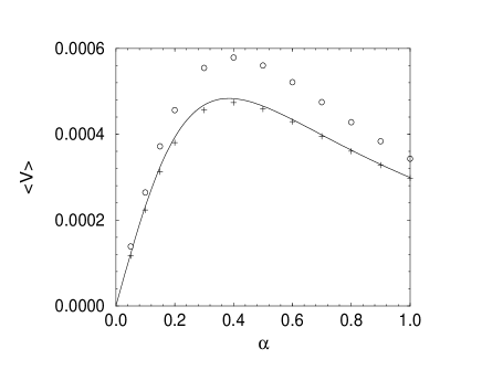
Figure 2: Mean kink velocity versus the damping coefficient. Parameters are $\lambda=-0.5$, $\epsilon=0.1$, $\omega=0.4$, $\theta_{0}=\pi/2$. The solid line represents the approximated solution of the CC theory (Eq. (17)); whereas circles and pluses are the results of the numerical simulations of the PDE (1) and the numerical solutions of the CC equations (6)-(6b), respectively.

In Fig. 2 we show the same dependence for an higher value of the driver frequency ($\omega=0.4$). We see that although the approximated solution (17) and the numerical solution of the CC equations are quite close, there is a discrepancy with the PDE results starting from the peak and extending to higher values of $\alpha$, this indicating that the CC ansatz is valid only for $\omega<<\omega_{ph}$ ($\omega_{ph}=1.2699$ for $\lambda=-0.5$).

In Fig. 3, we check Eq. (18) for the optimal value $\alpha_{opt}(\omega)$ of the damping constant for $\lambda=-0.5$. We can see that this value increase up to $\omega\approx 0.7$ and after that $\alpha_{opt}(\omega)$ decreases. Again, a good agreement between the CC theory and PDE results is found at small $\omega$ values.

By increasing the amplitude $\epsilon$ of the driver, reversal of current can also occur mn . This is shown in Fig. 4 from which we see that as $\alpha$ is increased the mean velocity computed from PDE simulations displays a crossover from negative to positive values (i.e. a current reversal occurred). This phenomenon is described neither by the CC analysis (notice that Eq. (17) predicts a positive average velocity for all $\lambda<0$), nor by the numerical solutions of the CC analysis depicted in the figure. This agrees with the claim made in Ref. mn that reversal currents do not depend on the internal mode mechanism, but rather on the existence of phonons in the system. In order to show the presence of phonon modes when this phenomenon appears, we have plotted in Fig. 5 the discrete Fourier Transform (DFT) of the kink’s width $W(t)$ (obtained from the numerical simulations of the PDE equation) for two values of $\alpha$, i.e. $\alpha=0.2$ (before crossover occurs) and $\alpha=0.7$ (inside the rectified motion region). In the former case (upper panel), one of the frequencies of the oscillations of $W(t)$ lies inside the phonon band, so phonons are clearly excited. In the latter case (lower panel) the main frequencies of the spectrum are well below the lower phonon edge ($w_{ph}/(2\pi)\approx 0.2$). From this we conclude that phonon modes are important for current reversals and a theory based on the internal mode alone (as the one presented here) cannot describe properly this phenomenon.

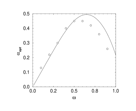
Figure 3: Optimal value of the damping as a function of the frequency of the ac force for $\lambda=-0.5$. The solid line represents the results obtained from Eq. (18) while the circles refer to numerical simulations of Eq. (1).

Figure 4: Mean kink velocity versus the damping coefficient for $\lambda=-0.5$; $\epsilon=0.5$, $\omega=0.4$, $\theta_{0}=\pi/2$. The solid line represents the approximated solution of the CC theory (Eq. (17)) while circles and pluses denote the results of the numerical simulations of the PDE (1) and of the numerical solutions of the CC equations (6)-(6b), respectively. The PDE results show that for very small values of damping ($\alpha<0.1$) pairs of kink and antikink appear.

Figure 5: DFT of the width of the kink, $W(t)$, obtained from the numerical solutions of the PDE for the same parameters of Fig. 4 and $\alpha=0.1$ (upper panel) and $\alpha=0.7$ (lower panel, when the current is rectified). The upper panel refers to the case in which a current reversal occours. The relevant frequencies in the spectrum are: $\omega_{1}=2\omega=0.8$; $\omega_{2}=3\omega=1.2$; $\omega_{3}=\omega=0.4$ and $\omega_{4}=(7/2)\omega=1.4$ (this last being inside the phonon band). The lower panel correspond to the case in which the current is rectified. The main frequencies in this case are located at $\omega_{1}=\omega=0.4$ and $\omega_{2}=2\omega=0.8$ away from the phonon’s band. The frequency of the internal mode and the lower phonon’s frequency are $\Omega_{I}=1.056$ and $\omega_{ph}=1.269$, respectively.

In Ref. mn a resonant behavior of mean velocity as a function of $\omega$ was also reported (see the peak of $\langle V\rangle$ at $\omega\approx\Omega_{I}$ in Fig. 3 of this paper). This feature is also confirmed by Eq. (17) (notice that the denominator of this expression has a minimum at $\omega=\Omega\approx\Omega_{I}$) although, in this case, the agreement with PDE results is only qualitative. This is shown in Fig. 6 from which we see the presence of a resonant structure, with good agreement at small frequencies and large deviations from PDE results at higher $\omega>0.6$ values. The agreement at low frequencies can be understood from the fact that phonons in this case are hardly excited and the CC description becomes accurate. On the contrary, when $\omega$ gets close to the resonant peak, phonons are easily excited and the CC analysis becomes unadequate.

We have also investigated the dependence of the phenomenon on the asymmetry parameter $\lambda$ as well as the importance of the damping term for soliton ratchets. In Fig. 7 we show the mean velocity as a function of $\lambda$ for fixed system parameters and two different values of $\alpha$. We see that the curve is anti-symmetric around the origin meaning that the sign of $\lambda$ determines the direction of motion, the maximal effect occurring around $|\lambda|=0.5$, i.e. the point of maximal asymmetry of the potential.

Finally, we have investigated the zero damping limit of the phenomenon. In Fig.8 we depict the time evolution of the center of mass of the kink for $\alpha=0$ and for different values of the initial condition phase $\theta_{0}$ of the ac force. We see that $X(t)$ is basically a linear function of time, whose slope depends on $\cos(\theta_{0})$. This implies that, in this case, is the initial phase which determines the direction of the motion and not only the asymmetry of the potential, as predicted by the CC analysis. Since in most experimental contexts initial phase are usually unknown, one must consider the phase as a random variable and take average on it. This obviously implies that soliton ratchets cannot exist in the zero-damping limit.

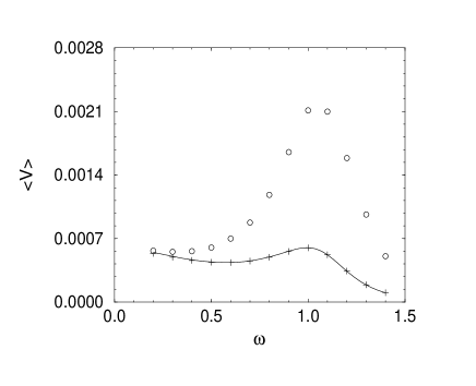
Figure 6: Mean velocity of the kink as a function of $\omega$. The pluses superimposing the solid line show a good agreement between the approximated (solid line) and the numerical (pluses) solutions of the CC theory. Results obtained from the integration of the Eq. (1) (circles) coincide with the CC theory only for smaller values of $\omega$. Parameters are fixed as $\lambda=-0.5$, $\epsilon=0.1$, $\theta_{0}=\pi/2$ and $\alpha=0.5$.

Figure 7: Mean velocity of the kink center of mass versus $\lambda$ for $\epsilon=0.1$, $\omega=0.1$, $\theta_{0}=\pi/2$ and for two values of the damping coefficient: $\alpha=0.2$ and $\alpha=0.5$ (for fixed $\lambda$, the mean velocity of the $\alpha=0.5$ case is smaller).

Figure 8: Time evolution of the center of the kink for different values of initial phase, $\theta_{0}$, in the non damped case. Parameters are fixed as: $\lambda=-0.5$; $\epsilon=0.1$ and $\omega=0.4$. The solid and the dashed lines represent the numerical simulations of Eq. (1) and the numerical solutions of Eq.s (6)-(6b), respectively.

V IV. Conclusions

In this paper we have studied the ratchet dynamics of the kink solution of the ADSGE by using a collective coordinate approach with two collective variables, the center of mass and the width of the kink. For these variables we have obtained a system of ODEs from which we derived an approximated expression for the mean velocity of the kink as a function of the system parameters. We have confirmed that the CC approach is valid when phonons are not excited in the system, i.e. for small values of $\epsilon$ and for $\omega<<\omega_{ph}$. We have shown that for a proper description of soliton ratchets it is not enough to consider the kink as a point particle moving in a ratchet potential goldobin ; carapella , but it is crucial to include also the internal oscillations of the kink profile. In particular, we have shown that the net motion of the kink becomes possible when its internal and translational modes become effectively coupled (the effective coupling being possible only in presence of damping). We also showed that the asymmetry of the potential determines the direction of the motion and that in the zero-damping case the ratchet effect vanishes (i.e. it depends on initial conditions). The resonant behavior of the velocity as a function of frequency and damping was also investigated. We found that the mean velocity approach a maximum value when the frequency of the ac force goes to the internal mode frequency or when the damping coefficient approach its optimal value. Finally, we have shown that the occurrence of current reversal is related to the presence of phonons in the system rather than the coupling between the translational and the internal mode.

In conclusion, the results of our analysis confirm the internal mode mechanism for soliton ratchet proposed in Ref. mn and provide an approximate analytical description of the phenomenon.

- (1) M. O. Magnasco, Phys. Rev. Lett. 71, 1477 (1993); C. R. Doering, Il Nuovo Cimento 17, 685 (1995).
- (2) P. Hänggi and R. Bartussek, in Lecture notes in Physics, Ed.s J. Parisi et al., Springer, Berlin, 476 (1996).
- (3) S. Cilla, F. Falo, and L. M. Floría, Phys. Rev. E 63, 031110 (2001).
- (4) P. Reimann and P. Häggi, Appl. Phys. A75, 169 (2002).
- (5) F. Marchesoni, Phys. Rev. Lett. 77, 2364 (1996).
- (6) A.V. Savin, G.P. Tsironis, A.V. Zolotaryuk, Phys.Lett. A 229, 279 (1997); Phys. Rev. E 56, 2457 (1997).
- (7) F. Falo, P. J. Martínez, J. J. Mazo and S. Cilla, Europhys. Lett. 45, 700 (1999); E. Trías, J.J. Mazo, F. Falo, and T.P. Orlando, Phys. Rev. E 61, 2257 (2000).
- (8) L. P. Faucheux, L. S. Bourdieu, P. D. Kaplan and A. J. Libchaber, Phys. Rev. Lett. 74, 1504 (1995).
- (9) C. S. Lee, B. Jankó, I. Derényi and A. L. Barabási, Nature 440, 337 (1999).
- (10) G. Carapella and G. Costabile, Phys. Rev. Lett. 87, 077002 (2001).
- (11) P. Reimann, Phys. Rep. 361, 57 (2002).
- (12) R. Bartussek, P. Hänggi, and J. G. Kissner, Europhys. Lett. 28, 459 (1994).
- (13) P. Reimann, R. Bartussek, R. Häussler, P. Hänggi, Phys. Lett. A215, 26 (1996).
- (14) Mario Salerno and Niurka R. Quintero, Phys. Rev. E, 65 025602(R) (2002).
- (15) Mario Salerno and Yaroslav Zolotaryuk. Phys. Rev. E 65, 056603 (2002).
- (16) S. Flach, Y. Zolotaryuk, A. E. Miroshnichenko, and M. V. Fistul. Phys. Rev. Lett. 88, 184101 (2002).
- (17) Luis Morales-Molina, Niurka R. Quintero, Franz G. Mertens, and Angel Sánchez, Phys. Rev. Lett. (2003) (to appear).
- (18) G. Costantini, F. Marchesoni and M. Borromeo, Phys. Rev. E 65, 051103 (2002).
- (19) I. Zapata, R. Bartussek, F. Sols, and P. Häggi, Phys. Rev. Lett. 77, 2292 (1996).
- (20) Mario Salerno, Physica D17, 227 (1985).
- (21) M. J. Rice and E. J. Mele, Solid State Commun. 35, 487 (1980); Mario Salerno and Alwyn C. Scott, Phys. Rev. B 26, 2474 (1982).
- (22) F. G. Mertens, H. J. Schnitzer, and A. R. Bishop, Phys. Rev. B 56, 2510 (1997); N.R. Quintero, A. Sánchez and F. Mertens, Phys. Rev. E 62, 5695 (2000).
- (23) W. H. Press, S. A. Teukolsky, W. T. Vetterling and B. P. Flannery, Numerical Recipes in Fortran 2nd Edition, Cambridge University Press (1992).
- (24) IMSL MATH/LIBRARY Special Functions. Visual Numerics, Inc., Houston, TX 77042 USA.
- (25) E. Goldobin, A. Sterck, and D. Koelle, Phys. Rev. E 63, 031111 (2001).