Characteristics of a Delayed System with Time-dependent Delay Time

Abstract

The characteristics of a time-delayed system with time-dependent delay time is investigated. We demonstrate the nonlinearity characteristics of the time-delayed system are significantly changed depending on the properties of time-dependent delay time and especially that the reconstructed phase trajectory of the system is not collapsed into simple manifold, differently from the delayed system with fixed delay time. We discuss the possibility of a phase space reconstruction and its applications.

The effect of time delay due to a finite propagation speed of information is usually considered as the form of delay-differential equation: $\dot{x}=f(x(t),x(t-\tau_{0}))$, where $\tau_{0}$ is the fixed delay time Opt ; MG ; Bio ; Chem ; Cont ; Comm ; Measure ; Farmer ; TD_Sync ; Map_Delay ; TD_Recon ; Bunner . It has been found that the system actually exhibits many different behaviors depending on the nonlinearity and the delay of the system and that the dimension of the attractor rises linearly with the delay time, even though the number of degree of freedom is small Farmer ; TD_Sync ; Map_Delay ; TD_Recon . In the last decade, models based of delay time have been extensively investigated in various fields such as opticsOpt , biology MG ; Bio and chemistry Chem for the purpose of understanding its fundamental role and of applying it to control Cont and communication Comm ; Measure .

The models based on fixed delay time, however, often fail to properly cover such real factors as (a) memory effect of the oscillator, (b) approximately known delay time, and (c) time-dependent delay time Vol ; DDT1 ; DDT2 . To cover these factors, Volterra first proposed a model based on distributed delays Vol . The model has been used in various areas DDT1 ; DDT2 ; Vol_Area . It has been shown very recently that the distributed delay induces a death phenomenon in a much larger set of parameters than that of the fixed delay DDT2 . Thus the Volterra’s model has enabled us to understand the realistic effects of delay times in dynamical systems.

Meanwhile, in studying the population dynamics and epidemic problems the delay time has been considered as a function of state variable Hale and there have been extensive investigations in that direction. However, there are many real situations in which the dynamics of delay time can not be described by an analytic function, e.g., neural networks and internet DynTopo . So it is reasonable to introduce time-dependent delay time as a stochastic process in those cases. In this point of view we shall investigate the effects of time-dependent delay time (TDT) in dynamical systems governed by a stochastic process and the effects in time-delayed systems remain much less studied.

The main goal of this paper is to show how TDT alters the characteristics of time-delayed systems. In addition, we analyze these characteristics with regards to application to communication.

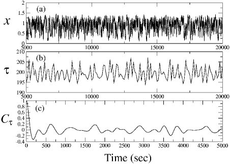
Figure 1: temporal behaviors of the modified Mackey-Glass model in the presence of TDT when $\tau_{0}=200$, $T=100$, and $\Lambda=10$: (a) state variable $x$; (b) the delay time; (c) autocorrelation of the time-dependent delay time.

We consider the modified Mackey-Glass model. The Mackey-Glass model MG was introduced as a model showing the regeneration of blood cells in patients suffering from leukemia. The modified Mackey-Glass model is given by,

$$\dot{x} = \frac{ax(t-\tau(t))}{1+x^{10}(t-\tau(t))}-bx(t),$$

$${\tau}(t) = \tau_{0}+\int^{t}_{0}\xi(s)ds,$$ (1)

where $a=0.2$, $b=0.1$. While in the Mackey-Glass model the delay time is a constant $\tau=\tau_{0}$, in the modified Mackey-Glass model $\tau$ is a function of time. Especially we focus on the case where $\tau(t)$ is governed by a stochastic process $\xi(t)$. As an example, we introduce the signal $\bar{\xi}(t)$ which is generated by the discrete sampling of the chaotic signal $x(t)$ such that $\bar{\xi}(t)=\frac{{x}(nT)-{x}((n-1)T)}{T}\Lambda$, when $t\in[nT,(n+1)T)$. We note that this form of the signal was taken for the convenience’s sake, which allows us to adjust the correlation length and modulation amplitude. And $\bar{\xi}$ actually exhibits quasi-stochastic signal because we shall study the sampling period of $T\in[100,1500]$ which is the larger than the correlation length of $x$ (the correlation length of x is $\tau_{x}\approx 70$ in the same parameters of Fig. 1. Our main results would not be changed if we use real stochastic signal for driving the delay time, because those results are related with the fact that the delay time is not determinable). Here, $\Lambda$ and $T$ are control parameters for the stochastic signal. They are proportional to the amplitude of $\tau(t)$ and its correlation length, respectively. The limit $\Lambda\rightarrow 0$ restores the system to the Mackey-Glass model. Figure 1 (a) and (b) show the temporal behavior of the modified Mackey-Glass model with TDT. In Fig. 1 (c), one see that the $\tau$ has the the correlation length of $O(T)$.

One of the most sensitive measures to detect the delay time of a system Measure ; TD_Recon is the one step prediction error Bunner . In the sufficiently small patch $U_{j}$ on $(x_{i},x_{i-\tau})$ plane, it is defined by $\sigma_{j}^{2}(\tau)=\frac{1}{N_{U_{j}}}\sum_{\vec{v}_{i}\in U_{j}}(\hat{\dot{x}}_{i}-g_{j}(\vec{v}_{i}))^{2}$, where $\vec{v}_{i}=(x_{i},x_{i-\tau})$ and $N_{U_{j}}$ are the numbers of data points in patch $U_{j}$. Here, $\hat{\dot{x}}=\frac{x(t+\delta t)-x(t)}{\delta t}$ is the time variation obtained from the observed signal $x(t)$. $\delta t$ is the sampling interval which should be much less than the characteristic time scale of the system (we took $\delta t=10^{-3}$). $g_{j}$ is a local linear function such that $g_{j}(\vec{v}_{j})=b_{j}+\vec{a}\cdot\vec{v_{j}}$, where the parameters $b_{j}$ and $\vec{a}_{j}$ are determined by the least square fitting. When this occurs, $\sigma_{j}$ is minimized Coeff . Therefore, the one step prediction error $\sigma$ is the average of the minimized $\sigma_{j}$, i.e., $\sigma=\langle\sigma_{j}\rangle$.

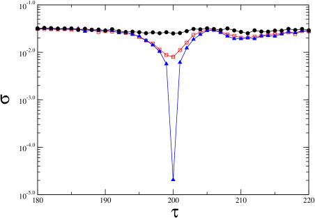
Figure 2: One step prediction errors for $\Lambda=0$ (filled triangle), $\Lambda=10$ (square), and $\Lambda=50$ (filled circle).

Figure 2 shows the one step prediction errors for the modified Mackey-Glass model depending on $\Lambda$. In the case of a fixed delay time (filled triangles) one can see that $\sigma$(which has a value of $\sigma=1.8\times 10^{-5}$) has a sharp peak at $\tau=200$. However, if the time dependency of delay time is turned on, i.e., $\Lambda\neq 0$, the depth of the peak decreases as the $\Lambda$ increases. Eventually, the peak almost disappears. At $\Lambda=50$ (filled circles) the prediction error has an almost constant value of $3.2\times 10^{-2}$. This means that if one detects the fixed delay time $\tau_{0}$, one can predict the time series $10^{3}$ times as precisely. As we shall see, it is closely related to the fact that the phase trajectory on the $(\dot{x}(t),x(t),x(t-\tau))$ space collapsed into the simple manifold. This is the crucial feature of the system based on the fixed delay time $\tau_{0}$. And Bünner et al. Bunner have shown that the delayed system can be modeled by the time delay embedding when $\tau_{0}$ is exactly detected. Meanwhile, in the case of TDT any detectable imprint is not left in the prediction error above the appropriate value of $\Lambda$. This feature indicates that the conventional modeling method for the delayed systems is not directly applicable.

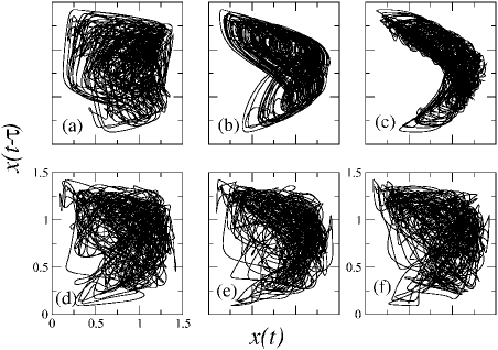
Figure 3: Reconstructed phase trajectories of the modified Mackey-Glass model in $(x(t),x(t-\tau))$ space:(a)-(c) fixed delay time ($\Lambda=0$); (d)-(f) time-dependent delay time ($\Lambda=50$). The reconstructions were performed at the lag time $\tau=190$((a) and (d)), $200$((b) and (e)), and $210$((c) and (f)), respectively.

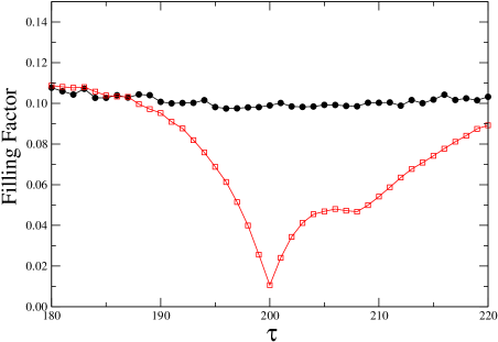
Figure 4: The filling factor as a function of lag time $\tau$. It is evaluated on $(x(t),x(t-\tau),\dot{x}(t))$ phase space when $\Lambda=0$ (circles) and $\Lambda=50$ (squares). We have taken the $10^{2}\times 10^{2}\times 10^{2}$ number of hypercubes for the region $x\in[0.0,2.0]$ , $x(t-\tau)\in[0.0,2.0]$, and $\dot{x}\in[-0.1,0.1]$ and we have iterated the systems during $5\times 10^{4}$ seconds for each point.

Figure 3 shows the reconstructed phase trajectories for fixed and TDTs in $(x(t),x(t-\tau))$ space. When the delay time is fixed (the first row of Fig. 3), the trajectory suddenly collapses into a quite simple shape at the value of $\tau=200$ (Fig. 3 (b)), while the others look very complex (we shall discuss the feature quantitively in the next paragraph). This explains why the prediction error sharply drops in the case of fixed delay time (filled triangles in Fig. 2). On the contrary, when the delay time is time-dependent (the second row of Fig. 3), one can not see any qualitative difference which coincides with the fact that the prediction error is almost constant in Fig. 2 (filled circles). This is a genuine effect caused by the nature of TDT. It presents a possibility that the delayed system with TDT can be used in communication with better performance.

To quantify the complexity of the attractors, we evaluate the filling factor which is the normalized number of hypercubes visited by the projected trajectory Bunner . It is one of the measures which directly show the complexity of the projected attractor. The results are presented in Fig. 4. In the case of TDT (filled circles in Fig. 4), the taken phase space is filled by $10\%$ and it hardly depends on the chosen time lag $\tau$ for reconstruction which explains the above description for Fig. 3 (d) - (f). In case of fixed time delay, if the time lag appropriately chosen as $\tau=200$, the attractor only fills $1\%$ of the taken phase space. Thus one may say that the reconstructed attractor of Fig. 2 (e) is 10 times as complex as that of Fig. 2 (b) based the values of the filling factors.

Figure 5: Average mutual information of the modified Mackey-Glass model: (a) fixed delay time ($\Lambda=0$) and (b) TDT at $\Lambda=270$.

In order to perform phase space reconstruction, the first step one must take is to find out the lag time $\tau_{e}$ for the delayed coordinates Taken ; Aba . It is usually determined by the first minimum point of the average mutual information. The average mutual information is defined by Mut_Info

$$I(\tau) = \sum_{x(n),x(n+\tau)}P(x(n),x(n+\tau))$$ (2)

$$\times\log_{2}\left[\frac{P(x(n),x(n+\tau))}{P(x(n))P(x(n+\tau))}\right].$$

Figure 5 shows the average mutual information in the cases of fixed delay and TDT. For the fixed delay time, the average mutual information has a peak near $\tau=200$, which has the same implication with that of the prediction error in Fig. 2. On the other hand, for TDT, the average mutual information has the delta function shape. This means that the information of the observed time series deteriorates more rapidly by TDT, compared to that of the fixed delay. Both of them have a wide range of degenerated minimum. In the latter, one can expect that the delay coordinate for phase space reconstruction would not be so unique because the degenerated region is wider than that of the former.

To analyze the global effects of the system according to the property of the driving signal, we consider the metric entropy defined by $h=\sum_{x(n)}P(x(n))\log_{2}[1/P(x(n))]$ which is a measure of complexity or strength of nonlinearity of the system Map_Delay . It corresponds to the value of the average mutual information $I(\tau)$ at $\tau=0$. Figure 6 shows the entropy as a function of $T$ and $\Lambda$. The value of entropy increases as $\Lambda$ and $1/T$ both increase, while in the delayed system with a fixed delay time it is almost constant Map_Delay . Therefore, we understand that the profile of TDT plays a significant role that controls the complexity and nonlinearity of the time-delayed system. All observations lead us to conclude that the nonlinearity characteristics of the time-delayed system are significantly changed depending on the properties of time-dependent delay time and, especially, that the reconstructed phase trajectory of the system is not collapsed into simple manifold, differently from the delayed system with fixed delay time.

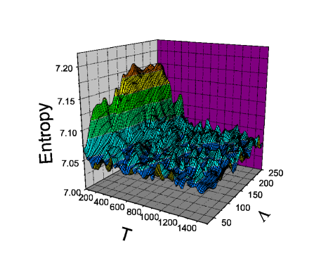
Figure 6: Entropy of the modified Mackey-Glass model as a function of $T$ and $\Lambda$

In conclusion, we have studied the characteristics of the time-delayed system in the presence of TDT. By presenting the numerical evidence, we have shown that the time-delayed system with TDT transits to the uncollapsible hyperchaotic system. This fact implies that the phase space reconstruction of the systems with TDT is hardly possible. The reason is that phase reconstruction methods for a time-delayed system usually assume the exact determination of fixed delay time TD_Recon ; Bunner . We expect that these characteristics of the time-delayed system with TDT should be useful to implement communication systems.

The authors thank M.-W. Kim and S.-Y. Lee for helpful discussions. This work is supported by Creative Research Initiatives of the Korean Ministry of Science and Technology.

References

- (1) K. Ikeda, Opt. Commun. 30, 257 (1979); G. Giacomelli, R. Meucci, A. Politi, and F.T. Arecchi, Phys. Rev. Lett. 73, 1099 (1994); V. Ahlers, U. Parlitz, and W. Lauterborn, Phys. Rev. E 58, 7208 (1998); A. Hohl, A. Gavrielides, T. Erneux, and V. Kovanis, Phys. Rev. A 59, 3941 (1999); G. Kozyreff, A.G. Vladimirov, and P. Mandel, Phys. Rev. E 64, 016613 (2001); T. Heil, I. Fischer, W. Elsas̈ser, J. Mulet, and C.R. Mirasso, Phys. Rev. Lett. 86, 795 (2001).
- (2) M.C. Mackey and L. Glass, Science 197, 287 (1977).
- (3) J. Fort and V. Meńdez, Phys. Rev. Lett. 89, 178101, (2002); S. Kunec and A. Bose, Phys. Rev. E 63, 021908 (2001).
- (4) I.R. Epstein, J. Chem. Phys. 92, 1702 (1990); P. Parmananda and J. L. Hudson, Phys. Rev. E 64, 037201 (2001); M. Bertram and A. S. Mikhailov, Phys. Rev. E 63, 066102 (2001).
- (5) K. Pyragas, Phys. Rev. Lett. 86, 2265 (2001); O.Lüthje, S. Wolff, and G. Pfister, Phys. Rev. Lett. 86, 1745 (2001).
- (6) B. Mensour and A. Longtin, Phys. Lett. A 224, 59 (1998); L.Yaowen, G. Guangming, Z. Hong, W. Yinghai, and G. Liang, Phys. Rev. E 62, 7879 (2000); V. S. Udaltsov, J.-P. Goedgebuer, L. Larger, and W.T. Rhodes, Phys. Rev. Lett. 86, 1892 (2001).
- (7) V.I. Ponomarenko and M.D. Prokhorov, Phys. Rev. E. 66, 026215 (2002). O. Lüthje, S. Wolf, and G. Pfister, Phys. Rev. Lett. 86, 1745 (2001).
- (8) T. Buchner and J. J. Źebrowski, Phys. Rev. E 63, 016210 (2000).
- (9) J.D. Farmer, Physica D 4, 366 (1982); T. Buchner and J.J. Zebrowski. Phys. Rev. E 63, 016210 (2000).
- (10) R. He and P.G. Vaidya, Phys. Rev. E 59, 4048 (1999); L. Yaowen, G, Gguangming, Z. Hong, and W. Yinghai, Phys. Rev. E 62, 7898 (2000).
- (11) B.P. Bezruchko, A.S. Karavaev, V.I. Ponomarenko, and M.D. Prokhorov, Phys. Rev. E 64, 056216 (2001).
- (12) M.J. Bünner, Th. Meyer, A. Kittel, and J. Parisi, Phys. Rev. E 56, 5083 (1997); R. Hegger, M.J. Bünner, H. Kantz, and A. Giaquinta, Phys. Rev. Lett. 81, 558 (1998); M.J. Bünner, M. Ciofini, A. Giaquinta, R. Hegger, H. Kantz, R. Meucci and A. Politi, Eur. Phys. J. D 10, 165 (2000).
- (13) V. Volterra, Lecons sur la théorie mathematique de la lutter pour la vie (Gauthiers-Villars, Paris, 1931).
- (14) F. Ghiringhelli and M.N. Zervas, Phys. Rev. E 65, 036604 (2002).
- (15) F.M. Atay, Phys. Rev. Lett. 91, 094101 (2003) and references therein.
- (16) N. MacDonald, Time Lags in Biological Models, Lecture Notes in Biomathematics Vol. 27 (Springer, Berlin, 1978); K. Gopalsamy, Stability and Oscillations in Delay Differential Equations of Population Dynamics (Kluwer Academic Publishers, Dordrecht, The Netherlands, 1992).
- (17) J.K. Hale, Theory of Functional Differential Equations, Springer-Verlag, Berlin, (1997) and references therein.
- (18) M.E.J. Newman, SIAM Review 45, 167-256 (2003); R. Albert, A.-L. Barabasi, Rev. Mod. Phys. 74, 47 (2002).
- (19) By applying the extremal conditions to the prediction error: and , one obtain three equations: , , , where . One can easily determine the parameters and for least square fitting by solving above equations.
- (20) F. Takens, in Dynamical Systems and Turbulence, Warwick 1980, Lecture Notes in Mathematics, edited by D.A. Rand and L.-S. Young (Springer-Verlag, Berlin, Heidelberg, 1980), Vol. 898, pp. 366-381; T. Sauer, J.A. Yorke, and M. Casdagli, J. Stat. Phys. 65, 579 (1991).
- (21) H.D.I Abarbanel, Analysis of Observed Chaotic Data, (Springer-Verlag New York, 1996).
- (22) A.M. Fraser and H.L. Swinney, Phys. Rev. A 33, 1134 (1986).