The Polymer Stress Tensor in Turbulent Shear Flows

Abstract

The interaction of polymers with turbulent shear flows is examined. We focus on the structure of the elastic stress tensor, which is proportional to the polymer conformation tensor. We examine this object in turbulent flows of increasing complexity. First is isotropic turbulence, then anisotropic (but homogenous) shear turbulence and finally wall bounded turbulence. The main result of this paper is that for all these flows the polymer stress tensor attains a universal structure in the limit of large Deborah number ${{\mathcal{D}}}\mkern-3.1mue\gg 1$. We present analytic results for the suppression of the coil-stretch transition at large Deborah numbers. Above the transition the turbulent velocity fluctuations are strongly correlated with the polymer’s elongation: there appear high-quality “hydro-elastic” waves in which turbulent kinetic energy turns into polymer potential energy and vice versa. These waves determine the trace of the elastic stress tensor but practically do not modify its universal structure. We demonstrate that the influence of the polymers on the balance of energy and momentum can be accurately described by an effective polymer viscosity that is proportional to to the cross-stream component of the elastic stress tensor. This component is smaller than the stream-wise component by a factor proportional to ${{\mathcal{D}}}\mkern-3.1mue^{2}$. Finally we tie our results to wall bounded turbulence and clarify some puzzling facts observed in the problem of drag reduction by polymers.

I Introduction

The dynamics of dilute polymers in turbulent flows is a rich subject, combining the complexities of polymer physics and of turbulence. Besides fundamental questions there is a significant practical interest in the subject, particularly because of the dramatic effect of drag reduction in wall bounded turbulent flows 49Tom ; 75Vir ; 90Gen ; 00SW . On the one hand the polymer additives provide a channel of dissipation in addition to the Newtonian viscosity; this had been stressed in the past mainly by Lumley 69Lum ; 72Lum . On the other hand the polymers can store energy in the form of elastic energy; this aspect had been stressed for example by Tabor and De Gennes 86TG . A better understanding of the relative roles of these aspects requires a detailed analysis of the dynamics of the “complex fluid” obtained with dilute polymers in the turbulent flow regime.

Some important progress in the theoretical description of the statistics of polymer stretching in homogeneous, isotropic turbulence of dilute polymer solutions was offered in Refs. 00Che ; 00BFL ; 01BFL . Here we want to stress the fact that in the practically interesting turbulent regimes, and in particular when there exists a large drag reduction effect, the characteristic mean velocity gradient (say, the mean shear, $S_{0}$), is much larger than the inverse polymer relaxation time, $\tau_{\rm{p}}$, $S_{0}\tau_{\rm{p}}\gg 1$. Usually this parameter is referred to as the Deborah or Weissenberg number:

$${{\mathcal{D}}}\mkern-3.1mue\equiv{\mathcal{W}}\!i\equiv S_{0}\tau_{\rm{p}}\ .$$ (1)

Indeed, the onset of drag reduction corresponds to Reynolds number ${{\mathcal{R}}}\mkern-3.1mue_{\rm{cr}}$ at which ${{\mathcal{D}}}\mkern-3.1mue\sim 1$. Large drag reduction corresponds to ${{\mathcal{R}}}\mkern-3.1mue\gg{{\mathcal{R}}}\mkern-3.1mue_{\rm{cr}}$ at which ${{\mathcal{D}}}\mkern-3.1mue\simeq{{\mathcal{R}}}\mkern-3.1mue/{{\mathcal{R}}}\mkern-3.1mue_{\rm{cr}}\gg 1$.

The aim of this paper is to provide a theory of the polymer stress tensor $\bm{\Pi}$ [defined in Eq. (3b)] in turbulent flows in which ${{\mathcal{D}}}\mkern-3.1mue\gg 1$. The main result is a relatively simple form (2a) of the mean polymer stress tensor $\bm{\Pi}_{0}$ that enjoys a high degree of universality. Denoting by $\widehat{\bf{x}}$ and $\widehat{\bf{y}}$ the unit vectors in the mean velocity and mean velocity gradient directions (streamwise and cross-stream directions in a channel geometry) and by $\widehat{\bf{z}}=\widehat{\bf{x}}\times\widehat{\bf{y}}$ the span-wise direction, we show that tensor $\bm{\Pi}_{0}$ has a universal form:

$$\bm{\Pi}_{0}\simeq\Pi^{yy}_{0}\left(\begin{array}[]{ccc}2{{\mathcal{D}}}\mkern-3.1mue^{2}&~{}{{\mathcal{D}}}\mkern-3.1mue{}&~{}~{}0{}{}\\ {{\mathcal{D}}}\mkern-3.1mue&1&0\\ 0&0&C\end{array}\right)\quad\mbox{for}\ {{\mathcal{D}}}\mkern-3.1mue\gg 1\ .$$ (2a)

One sees that in the ($$\widehat{\bf{x}} \widehat{\bf{y}} \bm{\Pi}_{0}$$-)-plane the tensorial structure of is independent of the statistics of turbulence:

$$\Pi^{xx}_{0}=2\,{{\mathcal{D}}}\mkern-3.1mue^{2}\Pi^{yy}_{0}\,,\qquad\Pi^{xy}_{0}=\Pi^{yx}_{0}={{\mathcal{D}}}\mkern-3.1mue\,\Pi^{yy}_{0}\ .$$ (2b)

Due to the to the symmetry of the considered flows with respect to reflection $$z\to-z \Pi_{0}^{xz} \Pi_{0}^{yz}$$, the off-diagonal components and vanish identically:

$$\Pi_{0}^{xz}=\Pi_{0}^{yz}=0\ .$$ (2c)

The only non-universal entry in Eq. (2a) is the dimensionless coefficient $C$. We show that $C=1$ for shear flows in which the extension of the polymers is caused by temperature fluctuations and/or by isotropic turbulence. For anisotropic turbulence the constant $C$ is of the order of unity.

The universal tensorial structure (2) has important consequences for the problem of drag reduction in dilute polymeric solutions. We show that the effect of the polymers on the balance of energy and mechanical momentum can be described by an effective polymer viscosity that is proportional to the cross-stream component of the elastic stress tensor $\Pi_{0}^{yy}$. According to Eq. (2b) this component is smaller than the stream-wise component $\Pi_{0}^{xx}$ by a factor of $2\,{{\mathcal{D}}}\mkern-3.1mue^{2}$. This finding resolves the puzzle of the linear increase of the effective polymeric viscosity with the distance from the wall, while the total elongation of the polymers [dominated by the largest component $\Pi^{xx}_{0}$ of the tensor (2a)] decreases with the distance from the wall. We show that our results for the profiles of the components $\Pi^{ij}_{0}$ are in a good agreement with DNS of the FENE-P model in turbulent channel flows.

The paper is organized as follows. In Sec. II.1 we present the basic equations of motion of the problem. In Sec. II.2 we describe the standard Reynolds decomposition of the equations of motion for the mean and fluctuations of the relevant variables. In Sec. II.3 we find general solution for $\bm{\Pi}_{0}$ and formulate (the very weak) conditions at which it simplifies to the universal form (2).

In Section III we analyze the phenomenon of polymer stretching in shear flows with prescribed turbulent velocity fields, either isotropic, Sec. III.2, or anisotropic, Sec. III.3. We relate the value of $C$ to the level of anisotropy in the turbulent flow. We also show in this section that a strong mean shear suppresses the threshold value for the coil-stretched transition by a factor ${{\mathcal{D}}}\mkern-3.1mue^{2}$, see Eqs. (27).

Sections IV and V are devoted to the case of strong turbulent fluctuations for which the fluctuating velocity and polymeric fields are strongly correlated. In Sec. IV we consider the case of homogeneous shear flows. In Sec. V we discuss wall bounded turbulence in a channel geometry, compare our results with available DNS data and apply our finding to the problem of drag reduction by polymeric solutions.

Section VI presents summary and a discussion of the obtained results .

Appendix A offers some useful exact relationships for the energy balance in the system.

II Equations of Motion and Solution for Simple Flows

II.1 Equations of motion for dilute polymer solutions

The equation for the velocity field of the complex fluid

reads:

$$\frac{\partial\,\bm{V}}{\partial t}+\left(\bm{V}\cdot\bm{\nabla}\right)\bm{V} = \nu_{0}\Delta\bm{V}-\bm{\nabla}P+\bm{\nabla}\cdot\bm{\Pi}\,,$$

$$\bm{\nabla}\cdot\bm{V} = 0\ .$$ (3a)

Here $$\bm{V}\equiv\bm{V}(t,\bm{r}) P\equiv P(t,\bm{r}) \nu_{0} \bm{\Pi}\equiv\bm{\Pi}(t,\bm{r})$$, and are the fluid velocity, the pressure, and Newtonian viscosity of the neat fluid respectively. The fluid is considered incompressible, and units are chosen such that the density is 1. The effect of the added polymer appears in Eq. (3a) via the elastic stress tensor .

In this paper we consider dilute polymers in the limit that their extension due to interaction with the fluid is small compared with their chemical length. In this regime one can safely assume that the polymer extension is proportional to the applied force (Hook’s law). We simplify the description of the polymer dynamics assuming that the relaxation to equilibrium is characterized by a single relaxation time $\tau_{\rm{p}}$, which is constant at small extensions. In this case $\bm{\Pi}$ can be written as

$$\bm{\Pi}(t,{\bm{r}})\equiv\frac{\nu_{0\rm p}}{\tau_{\rm{p}}}\overline{\bm{R}(t,{\bm{r}})\bm{R}(t,{\bm{r}})}\,,$$ (3b)

where $\nu_{0\rm p}$ is polymeric viscosity for infinitesimal shear, and $\bm{R}$ is the polymer end-to-end elongation vector, normalized by its equilibrium value (in equilibrium $\overline{\bm{R}\bm{R}}=\bm{\delta}$). The average in Eq. (3b) is over the Gaussian statistics of the Langevin random force which describes the interaction of the polymer molecules with the solvent molecules at a given temprature, but not over the turbulent ensemble.

The equation for the elastic stress tensor $\bm{\Pi}$

has the form

$$\frac{\partial\,{\bm{\Pi}}}{\partial t}+(\bm{V}\cdot\bm{\nabla}){{\bm{\Pi}}} = \bm{S}\cdot{{\bm{\Pi}}}+{{\bm{\Pi}}}\cdot\bm{S}^{\scriptscriptstyle{\rm T}}-\frac{1}{\tau_{\rm{p}}}\left({{\bm{\Pi}}}-{\bm{\Pi}}_{\rm{eq}}\right)\,,$$

$$\bm{S}\equiv\left(\bm{\nabla}\bm{V}\right)^{\scriptscriptstyle{\rm T}}, \quad S^{ij}=\partial V^{i}/\partial x^{j}\,,$$ (3c)

$$\bm{\Pi}_{\rm{eq}}=\Pi_{\rm{eq}}\bm{\delta}\,, \quad\Pi_{\rm{eq}}\equiv\nu_{0\rm p}/\tau_{\rm{p}}\ .$$

Here $\bm{S}\equiv\bm{S}(t,\bm{r})$ is the velocity gradient tensor and $\bm{\delta}$ is unit tensor.

Choice of coordinates.

In this paper we consider both homogeneous and wall bounded shear flows. In both cases we choose the coordinates such that the mean velocity is in the $\widehat{\bf{x}}$ direction and the gradient is in the $\widehat{\bf{y}}$ direction. In wall bounded flows $\widehat{\bf{x}}$ and $\widehat{\bf{y}}$ are unit vectors in the streamwise and the wall normal directions:

$$\bm{V}_{0} \equiv \left\langle V\right\rangle=\bm{S}_{0}\cdot\bm{r}\,,\quad\bm{S}_{0}\equiv S_{0}\,\widehat{\bf{x}}\widehat{\bf{y}}\,,$$

$$\text{only}\ V_{0}^{x}=S_{0}\,y\neq 0\ \text{and}\ S_{0}^{xy}=S_{0}\neq 0\ .$$

The unit vector orthogonal to $\widehat{\bf{x}}$ and $\widehat{\bf{y}}$ (the span-wise direction in wall bounded cases) is denoted as $\widehat{\bf{z}}$.

II.2 Reynolds decomposition of the basic equations

In the following we need to consider separately the mean values and the fluctuating parts of the velocity, ${\bm{V}}(\bm{r},t)$, the velocity gradient ${\bm{S}}(\bm{r},t)$, and the elastic stress tensor $\bm{\Pi}(\bm{r},t)$ fields. We define the fluctuating parts via

$$\bm{V}=\bm{V}_{0}+\bm{v}\,,\quad\bm{S}=\bm{S}_{0}+\bm{s}\,,\quad{{\bm{\Pi}}}={{\bm{\Pi}}}_{0}+\bm{\pi}\,,\dots$$ (5)

All the mean quantities will be denoted with a “₀” subscript (e.g. the mean velocity $\bm{V}_{0}$), and all the fluctuating quantities by the lower-case letters $\bm{v}$, $p$, $\bm{\pi}$, $\bm{s}$, etc. These mean values are computed with respect to the appropriate turbulent ensemble. Note that the mean pressure in a homogeneous shear flow is zero, $P_{0}=0$, and all mean quantities (except the mean velocity $V_{0}^{x}=S_{0}\,y$, of course) are coordinate independent and, by definition, time independent.

II.2.1 Equations for the mean objects

The equation for the mean elastic stress tensor

$\bm{\Pi}_{0}$ follows from Eq. (3c):

$$\hskip-59.75095pt\left(\frac{D}{D\,t}+\frac{1}{\tau_{\rm{p}}}\right){\bm{\Pi}}_{0}=\bm{S}_{0}\cdot{\bm{\Pi}}_{0}+{\bm{\Pi}}_{0}\cdot\bm{S}_{0}^{\scriptscriptstyle{\rm T}}+\bm{Q}\,,$$ (6c)

$$\bm{Q}\equiv\frac{1}{\tau_{\rm{p}}}\,\bm{\Pi}_{\rm{eq}}+\bm{Q}_{\scriptscriptstyle\rm{T}}\,,$$

$$\hskip-4.26773pt\bm{Q}_{\scriptscriptstyle\rm{T}}\equiv\left\langle\bm{s}\cdot\bm{\pi}+\bm{\pi}\cdot\bm{s}^{\scriptscriptstyle{\rm T}}\right\rangle\,,$$

where $$\bm{\Pi}_{\rm{eq}} \langle\cdots\rangle$$ is given by Eq. (3c), and denotes an average with respect to the turbulent ensemble. In components:

$$\Big{(}\frac{D}{D\,t}+\frac{1}{\tau_{\rm{p}}}\,\Big{)}\Pi_{0}^{ij}=S_{0}^{ik}\Pi_{0}^{kj}+S_{0}^{jk}\Pi_{0}^{ki}+Q^{ij}\,,$$

$$Q^{ij}=\frac{1}{\tau_{\rm{p}}}\Pi_{\rm{eq}}\delta^{ij}+\left\langle s^{ik}\pi^{kj}+s^{jk}\pi^{ki}\right\rangle\ .$$ (6d)

Here $D/Dt$ is the mean substantial time derivative

$$\frac{D}{D\,t}\equiv\frac{\partial}{\partial t}+\bm{V}_{0}\cdot\bm{\nabla}=\frac{\partial}{\partial t}+S_{0}\,y\,\frac{\partial}{\partial x}\ .$$ (7)

The substantial derivative vanishes in the stationary case, when all the statistical objects are $t$- and $x$-independent.

The equation for the mean velocity

follows from Eq. (3a):

$$\frac{\partial V_{0}}{\partial t}=\frac{\partial}{\partial y}\left[\nu_{0}S_{0}-W^{xy}+\Pi_{0}^{xy}\right]\,,$$ (8)

were ${\bm{W}}$ is the Reynolds stress tensor:

$$W^{ij}\equiv\left\langle v^{i}v^{j}\right\rangle\ .$$ (9)

In the stationary case $\partial V_{0}/\partial t=0$ and Eq. (8) gives

$$\nu_{0}S_{0}-W^{xy}+\Pi_{0}^{xy}={\cal P}\,,$$ (10)

where constant of integration $\cal P$ has a physical meaning of the total momentum flux. The three terms on the LHS of Eq. (10) describe the viscous, inertial and polymeric contributions to $\cal P$. In a homogeneous-shear geometry all theses terms are $y$-independent constants, whereas in a channel geometry they depend on the distance to the wall. Notice, that Eq. (10) also can be considered as an equation for the balance of mechanical forces in the flow.

II.2.2 Equations for the fluctuations

The equations for the fluctuating parts $\bm{v}$ and $\bm{\pi}$ read:

$$\frac{D\,\bm{v}}{D\,t}=-\bm{S}_{0}\cdot\bm{v}+\nu_{0}\Delta\bm{v}-\bm{\nabla}p+\bm{\nabla}\cdot\left(\bm{\pi}-\bm{v}\bm{v}\right)\,,$$

(11a)

$$\left(\frac{D}{D\,t}+\frac{1}{\tau_{\rm{p}}}\right)\bm{\pi}=\bm{S}_{0}\cdot\bm{\pi}+\bm{\pi}\cdot\bm{S}_{0}^{\scriptscriptstyle{\rm T}}+\bm{s}\cdot{\bm{\Pi}}_{0}+{\bm{\Pi}}_{0}\cdot\bm{s}^{\scriptscriptstyle{\rm T}}$$

$$~{}~{}~{}~{}~{}~{}~{}~{}~{}~{}~{}~{}~{}~{}~{}~{}~{}~{}~{}~{}~{}~{}~{}~{}~{}~{}~{}~{}~{}~{}~{}~{}~{}+\bm{\Phi}_{\pi}\,,$$ (11b)

where $$\bm{\nabla}\cdot\bm{v}=0$$, and

$$\bm{\Phi}_{\pi} \equiv \left(\bm{s}\cdot\bm{\pi}+\bm{\pi}\cdot\bm{s}^{\scriptscriptstyle{\rm T}}\right)^{\widetilde{}}-\bm{\nabla}\cdot\bm{v}\bm{\pi}\ .$$ (11c)

Here $(\dots)^{\widetilde{}}$ denotes the “fluctuating part of” $(\dots)$.

II.3 Solutions for simple flow configurations

II.3.1 Implicit solution for shear flows

Note that the mean shear tensor $\bm{S}_{0}$ satisfies, besides the incompressibility condition ${\rm Tr}\,\{\bm{S}_{0}\}=S_{0}^{ii}=0$, one additional constraint

$$S^{ij}_{0}S^{jk}_{0}=0\ .$$ (12)

Remarkably, this property of $\bm{S}_{0}$ uniquely distinguishes shear flows from other possibilities (elongational or rotational flows): if (12) holds, one can always choose coordinates such that the only nonzero component of $\bm{S}_{0}$ is $S_{0}^{xy}=S_{0}$.

Having Eq. (12) consider Eq. (6c) in the stationary state:

$${\bm{\Pi}}_{0}=\tau_{\rm{p}}\left(\bm{S}_{0}\cdot{\bm{\Pi}}_{0}+{\bm{\Pi}}_{0}\cdot\bm{S}_{0}^{\scriptscriptstyle{\rm T}}+\bm{Q}\right)\ .$$ (13)

We can proceed to solve this equation implicitly, treating $\bm{Q}$ on the RHS as a given tensor, and solve the linear set of equation for $\bm{\Pi}_{0}$. In the considered geometry Eq. (13) is a system of 4 linear equations, and the solution is expected to be quite cumbersome. However, property (12) allows a very elegant solution of this system. Using (13) iteratively (i.e., substituting instead of $\bm{\Pi}_{0}$ on the RHS of Eq. (13) the whole RHS), we get

$${\bm{\Pi}}_{0} = 2\tau_{\rm{p}}^{2}\bm{S}_{0}\cdot{\bm{\Pi}}_{0}\cdot\bm{S}_{0}^{\scriptscriptstyle{\rm T}}+\tau_{\rm{p}}^{2}\left(\bm{S}_{0}\cdot\bm{Q}+\bm{Q}\cdot\bm{S}_{0}^{\scriptscriptstyle{\rm T}}\right)+\tau_{\rm{p}}\bm{Q}$$

$$+\tau_{\rm{p}}^{2}\left(\bm{S}_{0}^{2}\cdot\bm{Q}+\bm{Q}\cdot\left(\bm{S}_{0}^{2}\right)^{\scriptscriptstyle{\rm T}}\right)\ .$$

One sees that due to Eq. (12) the last term in this equation vanishes. Repeating this procedure once again, we obtain the exact solution of (13) in the form of a finite (quadratic) polynomial of the tensor $\bm{S}_{0}$:

$$\bm{\Pi}_{0}=2\,\tau_{\rm{p}}^{3}\,\bm{S}_{0}\cdot\bm{Q}\cdot\bm{S}_{0}^{\scriptscriptstyle{\rm T}}+\tau_{\rm{p}}^{2}\left(\bm{S}_{0}\cdot\bm{Q}+\bm{Q}\cdot\bm{S}_{0}^{\scriptscriptstyle{\rm T}}\right)+\tau_{\rm{p}}\bm{Q}\ .$$ (14a)

The individual components of the solution Eq. (14a) are given by:

$$\Pi^{xx}_{0} = \tau_{\rm{p}}\left(2\,{{\mathcal{D}}}\mkern-3.1mue^{2}\,Q^{yy}+2\,{{\mathcal{D}}}\mkern-3.1mue\,Q^{xy}+Q^{xx}\right)\,,$$

$$\Pi^{xy}_{0} = \tau_{\rm{p}}\left({{\mathcal{D}}}\mkern-3.1mue\,Q^{yy}+Q^{xy}\right)\,,$$ (14b)

$$\Pi^{yy}_{0} = \tau_{\rm{p}}Q^{yy}\,,\qquad\Pi^{zz}_{0}=\tau_{\rm{p}}Q^{zz}\,,$$

$$\Pi_{0}^{xz} = \Pi_{0}^{yz}=0\ .$$

Notice that the ${xz}$ and $yz$ components of $\bm{\Pi}_{0}$ vanish due to the symmetry of reflection $z\to-z$, which remains relevant in all the flow configurations addressed in this paper.

In the limit ${{\mathcal{D}}}\mkern-3.1mue\gg 1$ the tensorial structure (14b) can be simplified to the form (2) if

$$Q^{xy}\ll{{\mathcal{D}}}\mkern-3.1mue\,Q^{yy}\,,\quad Q^{xx}\ll{{\mathcal{D}}}\mkern-3.1mue^{2}\,Q^{yy}\ .$$ (15)

Indeed, in this case one can neglect the last two terms in $\Pi_{0}^{xx}$ and the second term in $\Pi_{0}^{xy}$ and obtain Eq. (2) with $C=Q^{zz}/Q^{yy}$.

II.3.2 Explicit solution for laminar homogeneous shear flows

The solution (14) allows further simplification in the case of laminar shear flow, in which $\bm{Q}_{\scriptscriptstyle\rm{T}}$ of Eq. (6c) vanishes, $\bm{Q}_{\scriptscriptstyle\rm{T}}=0$, and thus, according to Eqs. (6c) and (3c), the tensor $\bm{Q}$ becomes proportional to the unit tensor:

$$Q^{ij}=\frac{\Pi_{\rm{eq}}}{\tau_{\rm{p}}}\,\delta^{ij}\ .$$ (16)

With this relationship Eq. (14a) simplifies to

$$\bm{\Pi}_{0}=\Pi_{\rm{eq}}\left(\begin{array}[]{ccc}2{{\mathcal{D}}}\mkern-3.1mue^{2}+1&~{}{{\mathcal{D}}}\mkern-3.1mue{}&~{}~{}0{}{}\\ {{\mathcal{D}}}\mkern-3.1mue&1&0\\ 0&0&1\end{array}\right)\ .$$ (17)

Equation (17), in which $\Pi_{\rm{eq}}$ is given by Eq. (3c), is important in itself as an explicit solution for $\bm{\Pi}_{0}$ in the case of laminar shear flow. But more importantly, this equation together with Eq. (14) gives a hint regarding the tensorial structure of $\bm{\Pi}_{0}$ even in the presence of turbulence, when the coupling between the velocity and the polymeric elongation field, leading to the cross-correlation $\bm{Q}_{\scriptscriptstyle\rm{T}}$, cannot be neglected.

To see why the simple result (17) may be relevant also for the turbulent case, note first that the non-diagonal elements with $z$ projection, i.e. $\Pi_{0}^{xz}$ and $\Pi_{0}^{yz}$, are identically zero in general as long as the symmetry $z\to-z$ prevails. Second, for large Deborah numbers, ${{\mathcal{D}}}\mkern-3.1mue\gg 1$, the nonzero components in both Eqs. (17) and (14b) have three different orders of magnitude: $\Pi_{0}^{xx}\gg\Pi_{0}^{xy}\gg\Pi_{0}^{yy}\simeq\Pi^{zz}$. In other words, the tensor $\bm{\Pi}_{0}$ is strongly anisotropic, reflecting a strong preferential orientation of the stretched polymers along the stream-wise direction $\widehat{\bf{x}}$. The characteristic deviation angle (from the $\widehat{\bf{x}}$ direction) is of order $O(1/{{\mathcal{D}}}\mkern-3.1mue)$.

Notice that Eqs. (14) relate the polymeric stress tensor $\bm{\Pi}_{0}$ to the cross-correlation tensor $\bm{Q}_{\scriptscriptstyle\rm{T}}$, Eq. (6c). In its turn this tensor depends on the polymeric stretching, which is described by the same tensor $\bm{\Pi}_{0}$. Therefore, generally speaking, Eqs. (14) remains an implicit solution of the problem, which in general requires considerable further analysis. However, as we discussed above, Eq. (14a) is more transparent than the starting Eq. (6). In particular, if the tensor $\bm{Q}$ is not strongly anisotropic, the tensorial structure of $\bm{\Pi}_{0}$ is close to Eq. (17) for the laminar case. We will see below that this structure is indeed recovered under more general conditions.

In the following Sects. III and IV we will find explicit solutions for the elastic stress tensor in the presence of turbulence which share a structure similar to Eq. (17). Namely, for ${{\mathcal{D}}}\mkern-3.1mue\gg 1$ the leading contribution to each component of $\bm{\Pi}_{0}$ can be presented as Eq. (2), in which $C$, given by Eqs. (30) and (53), is some constant of the order of unity, depending on the anisotropy of turbulent statistics.

III Polymer stretching in the passive regime

III.1 Cross-correlation tensor $\bm{Q}_{\scriptscriptstyle\rm{T}}$ in Gaussian turbulence

When ${{\mathcal{D}}}\mkern-3.1mue\gg 1$ the characteristic decorrelation time of turbulent fluctuations, $\tau_{\rm{cor}}\lesssim 1/S_{0}$, is much smaller than the polymer relaxation time $\tau_{\rm{p}}$. Accordingly the turbulent fluctuations can be taken as $\delta$-correlated in time:

$$\left\langle s^{ij}(t)s^{i^{\prime}j^{\prime}}(t^{\prime})\right\rangle=\Xi^{ii^{\prime},jj^{\prime}}_{\rm{pas}}\delta(t-t^{\prime})\ .$$ (18)

This approximation is valid below the threshold of coil-stretched transition, when the polymers do not affect the turbulent statistics. This regime will be referred to as the “passive” regime. The fourth-rank tensor $\bm{\Xi}_{\rm{pas}}$ defined by Eq. (18) is symmetric with respect to permutations of the two first and two last indices, $\Xi^{ii^{\prime},jj^{\prime}}_{\rm{pas}}=\Xi^{i^{\prime}i,j^{\prime}j}_{\rm{pas}}$. Incompressibility leads to the restriction $\Xi^{ik,jk}_{\rm{pas}}=0$. Homogeneity implies $\Xi^{ii^{\prime},jj^{\prime}}_{\rm{pas}}=\Xi^{ii^{\prime},j^{\prime}j}_{\rm{pas}}$.

At this point we assume also Gaussianity of the turbulent statistics. Then the tensor $\bm{Q}_{\scriptscriptstyle\rm{T}}$ can be found using the Furutsu-Novikov decoupling procedure developed in Novikov ; Furutsu for Gaussian processes:

$$Q^{ij}_{\scriptscriptstyle\rm{T}}=\Xi^{ij,kk^{\prime}}_{\rm{pas}}\Pi_{0}^{kk^{\prime}}\ .$$ (19)

The cross-correlation tensor $\bm{Q}_{\scriptscriptstyle\rm{T}}$ is proportional to a presently undetermined stress tensor $\bm{\Pi}_{0}$. To find $\bm{\Pi}_{0}$ one has to substitute Eq. (19) into Eq. (6) or into its formal solution (17) and to solve the resulting linear system of four equations for the non-zero components of $\bm{\Pi}_{0}$: $\Pi^{xx}$, $\Pi^{yy}$, $\Pi^{zz}$ and $\Pi^{xy}=\Pi^{yx}$.

The resulting equations are quite cumbersome. The basic physical picture simplifies however in two limiting cases: i) isotropic turbulence, Sec. III.2, and ii) anisotropic turbulence in the limit of strong shear, Sec. III.3.

III.2 Isotropic turbulence

First we consider the simplest case of isotropic turbulence. In this case the tensor $\bm{\Xi}_{\rm{pas}}$ has the form

$$\Xi^{ii^{\prime},jj^{\prime}}_{\rm{pas}}=\Xi\left[\delta^{ii^{\prime}}\delta^{jj^{\prime}}-\frac{1}{4}\left(\delta^{ij}\delta^{i^{\prime}j^{\prime}}+\delta^{ij^{\prime}}\delta^{i^{\prime}j}\right)\right]\ ,$$ (20)

where $\Xi$ is a constant measuring the level of turbulent fluctuations. Using Eq. (20) in Eq. (19) for $\bm{Q}_{\scriptscriptstyle\rm{T}}$ one gets

$$\bm{Q}_{\scriptscriptstyle\rm{T}}=\Xi\left(\Pi_{0}\bm{\delta}-\frac{1}{2}\,\bm{\Pi}_{0}\right)\ .$$ (21)

Substituting this relationship into (6c) one gets a closed equation for $\bm{\Pi}_{0}$:

$$\Big{(}\frac{D}{D\,t}+\frac{1}{\widetilde{\tau}_{\rm{p}}}\Big{)}\bm{\Pi}_{0}\!\! = \!\!\bm{S}_{0}\cdot\bm{\Pi}_{0}+\bm{\Pi}_{0}\cdot\bm{S}_{0}^{\scriptscriptstyle{\rm T}}$$

$$+\left(\Xi\Pi_{0}+\frac{1}{\tau_{\rm{p}}}\Pi_{\rm{eq}}\right)\bm{\delta}\,,$$

$$\frac{1}{\widetilde{\tau}_{\rm{p}}} \equiv \frac{1}{\tau_{\rm{p}}}+\frac{\Xi}{2}\ .$$ (22b)

The stationary solution of Eq. (22) has the form

$$\bm{\Pi}_{0} = \Pi_{0}^{yy}\left(\bm{\delta}+\widetilde{\tau}_{\rm{p}}\left(\bm{S}_{0}+\bm{S}_{0}^{\scriptscriptstyle{\rm T}}\right)+2\widetilde{\tau}^{2}_{\rm{p}}\bm{S}_{0}\cdot\bm{S}_{0}^{\scriptscriptstyle{\rm T}}\right)\,,$$

$$\Pi_{0}^{yy} = {\widetilde{\tau}_{\rm{p}}}\left(\Xi\Pi_{0}+\frac{1}{\tau_{\rm{p}}}\Pi_{\rm{eq}}\right)\,,$$ (23a)

$$\Pi_{0} \equiv {\rm Tr}\,\{\bm{\Pi}_{0}\}\ .$$

In components:

$$\bm{\Pi}_{0} = \Pi_{0}^{yy}\left(\begin{array}[]{ccc}2\,\widetilde{{{\mathcal{D}}}\mkern-3.1mue}^{2}+1&~{}~{}\widetilde{{{\mathcal{D}}}\mkern-3.1mue}{}{}&~{}0{}\\ \widetilde{{{\mathcal{D}}}\mkern-3.1mue}&1&0\\ 0&0&1\end{array}\right)\,,$$ (23e)

$$\widetilde{{{\mathcal{D}}}\mkern-3.1mue} \equiv \widetilde{\tau}_{\rm{p}}\,S_{0}<{{\mathcal{D}}}\mkern-3.1mue\ .$$ (23f)

We see that the tensor structure of $\bm{\Pi}_{0}$ has the same form as in the laminar case, but with an increased relaxation frequency given by Eq. (22b).

Taking the trace of Eq. (23), one gets the following equation for $\Pi_{0}^{yy}$:

$$\Pi_{0}^{yy} = \frac{1}{\tau_{\rm{p}}}\,\Gamma\,\Pi_{\rm{eq}}\,,$$ (24)

$$\Gamma \equiv \frac{1}{\tau_{\rm{p}}}-\left(2\,\widetilde{{{\mathcal{D}}}\mkern-3.1mue}^{2}+\frac{5}{2}\right)\Xi\ .$$ (25)

We see that the effective damping $\Gamma$ decreases with increasing the turbulence level $\Xi$. At some critical value of $\Xi=\Xi_{\rm{c}}$, the effective damping goes to zero, $\Gamma\to 0$, and formally $\Pi_{0}\to\infty$. The critical value $\Xi_{\rm{c}}$ corresponds to the threshold of the coil-stretch transition. Substituting Eq. (23f) into the threshold condition $\Gamma=0$, one gets a 3rd-order algebraic equation for $X\equiv\Xi_{\rm{c}}\tau_{\rm{p}}$:

$$5X^{3}+18X^{2}+4(3+4\,{{\mathcal{D}}}\mkern-3.1mue^{2})X=8\ .$$ (26)

This equation has one real root $\Xi_{\rm{c}}$, which we consider in two limiting cases:

• Small shear $S_{0}\ll{1}/{\tau_{\rm{p}}}$ (${{\mathcal{D}}}\mkern-3.1mue\ll 1$). In this case the threshold turbulence level $\Xi_{\rm{c}}$ is proportional to the polymer relaxation frequency

  $$\Xi_{\rm{c}} \simeq \frac{2}{5\,{\tau_{\rm{p}}}}\left(1-\frac{5\,{{\mathcal{D}}}\mkern-3.1mue^{2}}{9}\right)\,.$$ (27a)

• Large shear $S_{0}\gg{1}/{\tau_{\rm{p}}}$ (${{\mathcal{D}}}\mkern-3.1mue\gg 1$). In this case the threshold velocity gradient is much smaller. Indeed:

  $$\Xi_{\rm{c}} \simeq \frac{1}{2\,\tau_{\rm{p}}\,{{\mathcal{D}}}\mkern-3.1mue^{2}}\left(1-\frac{3}{4\,{{\mathcal{D}}}\mkern-3.1mue^{2}}\right)\,.$$ (27b)

Evidently, the strong mean shear decreases the threshold of the coil-stretch transition very significantly, by a factor of ${{\mathcal{D}}}\mkern-3.1mue^{2}$. The important conclusion is that in the entire region below the threshold, $\Xi\leq\Xi_{\rm{c}}$, the renormalization of the Deborah number can be safely neglected:

$${{\mathcal{D}}}\mkern-3.1mue-\widetilde{{{\mathcal{D}}}\mkern-3.1mue}\leq\frac{1}{4\,{{\mathcal{D}}}\mkern-3.1mue}\ll 1\ .$$ (28)

This means that the structure of the elastic stress tensor in the passive regime (23e) hardly differs from the laminar case (17).

III.3 The elastic stress tensor in anisotropic turbulent field

Here we consider the case of strong shear, ${{\mathcal{D}}}\mkern-3.1mue\to\infty$, having in mind that in the passive regime the tensorial structure of $\bm{\Xi}_{\rm{pas}}$ [see Eq. (20)] is independent of ${{\mathcal{D}}}\mkern-3.1mue$. In this case the leading contributions to each component of $\bm{\Pi}_{0}$ in Eq. (14b) are:

$$\Pi^{xx}_{0} = 2\tau_{\rm{p}}\,{{\mathcal{D}}}\mkern-3.1mue^{2}\,Q^{yy}\,,$$

$$\Pi^{xy}_{0} = \tau_{\rm{p}}{{\mathcal{D}}}\mkern-3.1mue\,Q^{yy}\,,$$ (29)

$$\Pi^{yy}_{0} = \tau_{\rm{p}}Q^{yy}\,,\qquad\Pi^{zz}_{0}=\tau_{\rm{p}}Q^{zz}\,,$$

$$\Pi_{0}^{xz} = \Pi_{0}^{yz}=0\ .$$

This means that for ${{\mathcal{D}}}\mkern-3.1mue\gg 1$ $\bm{\Pi}_{0}$ takes on the form (2) with

$$C\simeq\frac{\Xi^{yy,xx}_{\rm{pas}}}{\Xi^{zz,xx}_{\rm{pas}}}\ .$$ (30)

The threshold condition for $\bm{\Xi}$ can be found along the lines of the preceding subsection. The result is that only one component of the tensor $\bm{\Xi}_{\rm{pas}}$ is important:

$$\Xi^{yy,xx}_{\rm{pas,c}}\simeq\frac{1}{2\,\tau_{\rm{p}}\,{{\mathcal{D}}}\mkern-3.1mue^{2}}\ .$$ (31)

This result coincides to leading order with Eq. (27b) in which $\Xi^{yy,xx}_{\rm{pas}}\Rightarrow\Xi$ according to Eq. (20).

Finally, we point out that the results presented in this section remain valid for finite, but small, decorrelation time $\tau_{\rm{cor}}\to 0$ in which $\Xi$ can be defined as $\Xi\equiv^{2}\sigma_{0}2\tau_{\rm{cor}}/15$, where $\sigma_{0}^{2}\equiv\left\langle(\partial^{\alpha}u^{\beta})2\right\rangle={\rm Tr}\,\left\langle\bm{s}\cdot\bm{s}^{\scriptscriptstyle\rm{T}}\right\rangle$.

Notice that experimental and numerical studies 75Vir ; 00SW ; DNS1 show that the level of turbulent activity in turbulent polymeric flows is of the same order as in Newtonian flow at the same conditions. Simple estimations for the typical conditions in the MDR regime, when one observes large drag reduction, show that the parameter $\Xi$ is far above the threshold value (27b). Therefore, polymers in the MDR regime cannot be considered as passive: there should be some significant correlations between polymers and fluid motion that prevent polymers from being infinitely extended despite of supercritical level of turbulence. The character of these correlations is clarified in the following Section.

IV Active regime of the polymer stretching

In this Section we continue the discussion of the case of homogeneous turbulence with mean shear, but allow for supercritical levels of turbulent fluctuations, at which the polymers are strongly stretched. In that case they can no longer be considered as a passive field that does not affect the turbulent fluctuations. In this active regime of the polymer stretching one cannot use Eq. (19) for the cross-correlation tensor $\bm{Q}_{\scriptscriptstyle\rm{T}}$ of the turbulent velocity field ${\bm{v}}(\bm{r},t)$ and polymeric stretching ${\bm{\pi}}(\bm{r},t)$. In the present Section we reconsider the $\bm{v}-\bm{\pi}$ correlations and show that in the active regime they are determined by the so-called hydroelastic waves which are involved in transforming turbulent kinetic energy into polymer potential energy and vice versa. Therefore in order to find $\bm{Q}_{\scriptscriptstyle\rm{T}}$ in the active regime we need first to study the basic properties of the hydroelastic waves themselves. This is done in Sects. IV.1 and IV.2. In Sec. IV.1 we demonstrate that the coupled Eqs. (34) for ${\bm{v}}$ and ${\bm{\pi}}$ give rise to propagating hydro-elastic plane waves

$$\bm{v}_{{\bm{k}}}\,,{\bm{b}}_{\bm{k}}\propto\exp[i\left({\bm{k}}\cdot\bm{r}-\omega_{\bm{k}}t\right)-\gamma_{k}t]$$ (32a)

with the dispersion law $$\omega_{\bm{k}} \gamma_{\bm{k}}$$ and damping :

$$\omega_{\bm{k}} = \sqrt{({\bm{k}}\cdot\bm{\Pi}_{0}\cdot{\bm{k}})}\,,\$$ (32b)

$$\gamma_{k} = \frac{1}{2}\left(\frac{1}{\tau_{\rm{p}}}+\nu_{0}k^{2}\right)\ .$$ (32c)

For large shear, ${{\mathcal{D}}}\mkern-3.1mue\gg 1$, these waves (with the exception of those propagating exactly in the stream-wise direction $\widehat{\bf{x}}$) have high quality-factor: $\omega_{\bm{k}}\gg\gamma_{k}$. The desired cross-correlation tensor $\bm{Q}_{\scriptscriptstyle\rm{T}}$ is defined by the polarization of the hydro-elastic waves, that is the subject of Sec. IV.2. In Sec. IV.3 we derive the following equation for tensor $\bm{Q}_{\scriptscriptstyle\rm{T}}$

$$Q_{\scriptscriptstyle\rm{T}}^{ij}=\Xi^{ij,kl}_{\rm{act}}\Pi^{kl}_{0}\,,$$ (33)

that is very similar to the corresponding Eq. (19) in the passive regime. However in Eq. (33) the proportionality tensor $\bm{\Xi}_{\rm{act}}$, given by Eq. (42), is very different from the corresponding tensor $\bm{\Xi}_{\rm{pas}}$ in the passive regime.

IV.1 Frequency and damping of hydro-elastic waves

The equations (11) for the vector $\bm{v}$ and tensor $\bm{\pi}$ can be reformulated in terms of a new vector:

$${\bm{b}}\equiv\tau_{\rm{p}}\bm{\nabla}\cdot\bm{\pi}\,,$$ (34a)

instead of the tensor $$\bm{\pi}$$. The new equations read

$$\mkern-50.0mu\frac{D\bm{v}}{D\,t} = -\bm{S}_{0}\cdot\bm{v}+\nu_{0}\Delta\bm{v}-\bm{\nabla}p+\gamma_{\rm{p}}\,{\bm{b}}+\bm{\mathcal{N}}_{v}\,,$$ (34b)

$$\mkern-50.0mu\frac{D{\bm{b}}}{D\,t} = -\frac{1}{\tau_{\rm{p}}}{\bm{b}}+\bm{S}_{0}\cdot{\bm{b}}-\tau_{\rm{p}}\widehat{\Omega}^{2}\,\bm{v}+\bm{\mathcal{N}}_{b}\,,$$ (34c)

where

$${\widehat{\Omega}}^{2} \equiv -\bm{\nabla}\cdot\bm{\Pi}_{0}\cdot\bm{\nabla}\,,$$ (34d)

$$\bm{\mathcal{N}}_{v} \equiv -\bm{\nabla}\cdot\bm{v}\bm{v}\,,\quad\bm{\mathcal{N}}_{b}\equiv\tau_{\rm{p}}\bm{\nabla}\cdot\bm{\Phi}_{\pi}\ .$$ (34e)

The linearized version of (34) gives rise to hydro-elastic waves steinberg ; 01BFL with an alternating exchange between the kinetic energy of the carrier fluid and the potential energy of the polymeric subsystem. In the simplest case of space-homogeneous turbulent media (no mean shear, $S_{0}=0$) the homogeneous Eqs. (34) have plane wave solutions cf. Eq. (32).

When the mean shear exists it appears in Eqs.  (34) with a characteristic frequency $S_{0}$. In the region of parameters that we are interested in, $S_{0}$ is much smaller than the wave frequency $\omega_{\bm{k}}$, but much larger than the wave damping frequency $\gamma_{k}$. This means that the shear does not affect the wave character of the motion, but it can change the effective damping of the plain wave with a given wave vector ${\bm{k}}$. Indeed, due to the linear inhomogeneity of the mean velocity (constant shear) the wave vector becomes time dependent according to

$$\frac{d{\bm{k}}}{dt}=-\bm{S}_{0}^{\scriptscriptstyle{\rm T}}\cdot{\bm{k}}\ .$$ (35)

This means that in the case $S_{0}\gg\gamma_{k}$ the shear frequency $S_{0}$ serves as an effective de-correlation frequency instead of $\gamma_{k}$:

$$\gamma_{\bm{k}}\Rightarrow\gamma=bS_{0}\,,$$ (36)

where $b$ is the dimensionless constant of the order of unity.

We reiterate that the limit ${{\mathcal{D}}}\mkern-3.1mue\gg 1$ is consistent with the frequency of the hydro-elastic waves $\omega_{\bm{k}}$ being much larger than their effective damping.

IV.2 Polarization of hydro-elastic waves

The formal solution of the linear Eq. (34c) for ${\bm{b}}$ can be written in terms of the Green’s function $\widehat{G}_{\rm{p}}$:

$${\bm{b}} = -\tau_{\rm{p}}\left(\widehat{G}_{\rm{p}}+\bm{S}_{0}\cdot\widehat{G}_{\rm{p}}^{2}\right)\widehat{\Omega}^{2}\,\bm{v}\,,$$ (37a)

$$\widehat{G}_{\rm{p}} \equiv \left(\frac{D}{D\,t}+\frac{1}{\tau_{\rm{p}}}\right)^{-1}\ .$$ (37b)

Denoting by $F_{n}(t,\bm{r})$ the result of $n$-fold action $\widehat{G}_{\rm{p}}^{n}$ on the function $f(t,\bm{r})$,

$$F_{n}(t,\bm{r})\equiv\widehat{G}_{\rm{p}}^{n}f(t,\bm{r})\,,$$ (38a)

one writes

$$F_{1}(t,\bm{r}) = \int\limits_{0}^{\infty}d\tau f(t-\tau,\bm{r}-\bm{S}_{0}\cdot\bm{r}\tau)\exp\left(-\frac{\tau}{\tau_{\rm{p}}}\right)\,,$$

$$F_{n}(t,\bm{r}) = \int\limits_{0}^{\infty}\frac{d\tau\,\tau^{n-1}}{(n-1)!}f(t-\tau,\bm{r}-\bm{S}_{0}\cdot\bm{r}\tau)\exp\left(-\frac{\tau}{\tau_{\rm{p}}}\right)\,.$$

By straightforward calculations one can show that $\widehat{G}_{\rm{p}}$ satisfies the following commutative relationship

$$\widehat{G}_{\rm{p}}\bm{\nabla}-\bm{\nabla}\widehat{G}_{\rm{p}}=\bm{S}_{0}^{\scriptscriptstyle{\rm T}}\cdot\widehat{G}_{\rm{p}}^{2}\bm{\nabla}\ .$$ (39)

Using this relation in Eq. (37a) repeatedly we can rewrite ${\bm{b}}$ as

$${\bm{b}} = \tau_{\rm{p}}\left[\left(\widehat{G}_{\rm{p}}\bm{\nabla}\cdot{\bm{\Pi}}_{0}\cdot\bm{\nabla}\right)+\bm{S}_{0}\cdot\left(\widehat{G}_{\rm{p}}^{2}\bm{\nabla}\cdot{\bm{\Pi}}_{0}\cdot\bm{\nabla}\right)\right]\bm{v}$$

$$= \tau_{\rm{p}}\Big{[}\left(\bm{\nabla}\cdot{\bm{\Pi}}_{0}\cdot\widehat{G}_{\rm{p}}\bm{\nabla}\right)+\left(\bm{\nabla}\cdot\bm{S}_{0}\cdot{\bm{\Pi}}_{0}\cdot\widehat{G}_{\rm{p}}^{2}\bm{\nabla}\right)$$

$$+\bm{S}_{0}\cdot\left(\bm{\nabla}\cdot{\bm{\Pi}}_{0}\cdot\widehat{G}_{\rm{p}}^{2}\bm{\nabla}\right)$$

$$+2\bm{S}_{0}\cdot\left(\bm{\nabla}\cdot\bm{S}_{0}\cdot{\bm{\Pi}}_{0}\cdot\widehat{G}_{\rm{p}}^{3}\bm{\nabla}\right)\Big{]}\bm{v}\,.$$

This is an exact relationship for the polarization of the hydro-elastic waves in the presence of mean shear, and it will be used in the analysis of the cross-correlation tensor $\bm{Q}_{\scriptscriptstyle\rm{T}}$.

IV.3 General structure of the cross-correlation tensor

The cross-correlation tensor $\bm{Q}_{\scriptscriptstyle\rm{T}}$ Eq. (6c) can be rewritten in terms of the vector field ${\bm{b}}$ as follows:

$$\bm{Q}_{\scriptscriptstyle\rm{T}}=-\frac{1}{\tau_{\rm{p}}}\left\langle\bm{v}{\bm{b}}+{\bm{b}}\bm{v}\right\rangle\ .$$ (41)

Substituting the vector ${\bm{b}}$ from Eq. (IV.2) into Eq. (41) one finds that the cross-correlation tensor $\bm{Q}_{\scriptscriptstyle\rm{T}}$ is proportional to the elastic stress tensor $\bm{\Pi}_{0}$, according to Eq. (33), in which the proportionality tensor $\bm{\Xi}_{\rm{act}}$ is expressed in terms of the second-order correlation functions of the velocity gradients, as follows:

$$\Xi^{ijkl}_{\rm{act}} = \Xi_{1}^{ijkl}+\Xi_{1}^{jikl}+\left(\Xi_{2}^{ijk^{\prime}l}+\Xi_{2}^{jik^{\prime}l}\right)S_{0}^{k^{\prime}k}$$

$$+\left(S_{0}^{jj^{\prime}}\Xi_{2}^{ij^{\prime}kl}+S_{0}^{ii^{\prime}}\Xi_{2}^{ji^{\prime}kl}\right)$$

$$+2\left(S_{0}^{jj^{\prime}}\Xi_{3}^{ij^{\prime}k^{\prime}l}+S_{0}^{ii^{\prime}}\Xi_{3}^{ji^{\prime}k^{\prime}l}\right)S_{0}^{k^{\prime}k}\ .$$

Here $$\bm{\Xi}_{n}$$ are time-integrated tensors defined as follows:

$$\bm{\Xi}_{n}\equiv\int_{0}^{\infty}\frac{d\tau\,\tau^{n-1}}{(n-1)!}\,{\bm{\Xi}}(\tau)\exp\left(-\frac{\tau}{\tau_{\rm{p}}}\right)\,$$ (42b)

$$\Xi^{ijkl}(\tau)\equiv\left\langle\frac{\partial v^{i}(t,\bm{r})}{\partial r^{k}}\frac{\partial v^{j}(t-\tau,\bm{r}^{\prime})}{\partial r^{{}^{\prime}l}}\right\rangle\$$ (42c)

and $\bm{r}^{\prime}=\bm{r}-\tau\,\bm{S}_{0}\cdot\bm{r}$.

In order to estimate the relative importance of $\Xi_{1}$, $\Xi_{2}$, and $\Xi_{3}$ in Eq. (42) notice that the integrals in Eq. (42b) are dominated by contributions from the longest hydro-elastic waves in the system. These longest $k$-vectors have a decorrelation time $\gamma$ [which is estimated in Eq. (36)], and are characterized by a frequency $\omega$ that we will be specified below. Using these estimates we can approximate the time dependence of $\Xi^{ijkl}(\tau)$ as follows

$$\Xi^{ijkl}(\tau) \Rightarrow \sigma^{ijkl}f(\tau)\,,\quad\bm{\sigma}\equiv\bm{\Xi}(0)$$ (43a)

$$f(\tau) = \cos\left(\omega\,\tau\right)\,\exp\left(-\gamma\tau\right)\ .$$ (43b)

Note that the assumption here is that $\omega$ and $\gamma$ do not depend on the tensor indices. This is a simplifying assumption that does not carry heavy consequences for the qualitative analysis.

Under these assumptions the tensors ${\bm{\Xi}}_{n}$ in Eq. (42) can be estimated as follows

$$\Xi^{ijkl}_{n} = f_{n}\sigma^{ijkl}\,,$$ (44a)

$$f_{n} = \int_{0}^{\infty}\frac{d\tau\,\tau^{n-1}}{(n-1)!}\,f(\tau)\exp\left(-\frac{\tau}{\tau_{\rm{p}}}\right)$$ (44b)

$$\simeq \frac{\text{Re}(\gamma+i\omega)^{n}}{\left(\gamma^{2}+\Omega^{2}\right)^{n}}\,,$$

$$f_{1} \simeq \frac{\gamma}{\Omega^{2}}\,,\quad f_{2}\simeq-\frac{1}{\Omega^{2}}\,,\quad f_{3}\simeq-\frac{3\,\gamma}{\omega^{4}}\ .$$ (44c)

At this point we need to estimate $\omega$. From Eq. (32b) we see that we need to take the largest of component of $\bm{\Pi}_{0}$, and smallest available $k$ vector which will be denoted as $k_{\rm min}$. Since we expect the $xx$ component of $\bm{\Pi}_{0}$ to be the largest component we write

$$\omega\simeq\sqrt{\Pi^{xx}_{0}}\,k_{\rm min}\ .$$ (45)

We should note at this point that homogeneous turbulence has no inherent minimal $k$ vector, since there is no natural scale. In reality there is always an outer scale which is determined by external constraints. For further progress in the analysis of the structure of the cross-correlation tensor one need to specify the outer scale of turbulence. To this end we will consider in the next Section homogeneous turbulence with a constant shear as an approximation to wall bounded turbulence of polymeric solution in the region of logarithmic mean velocity profile.

V Polymer stretching in wall bounded turbulence

In this section we consider turbulent polymeric solutions in wall bounded flows, and show that the elastic stress tensor takes on the universal form (2). This implies very specific dependence of the components of the elastic stress tensor on the distance from the wall. The theoretical predictions will be checked against numerical simulations and will be shown to be very well corroborated. Since we are interested in drag reduction we must consider here the active regime when the polymers are sufficiently stretched to affect the turbulent field. As mentioned before, large drag reduction necessarily implies ${{\mathcal{D}}}\mkern-3.1mue\gg 1$. For concreteness we restrict ourselves by considering the most interesting logarithmic-law region. Extension of our results to the entire turbulent boundary layer is straightforward.

V.1 Cross-correlation tensor in wall bounded turbulence

In this section we consider in more details tensor $\bm{Q}_{\scriptscriptstyle\rm{T}}$ for wall bounded turbulent flows. In this case the outer scale of turbulence is estimated as the distance to the wall. Therefore in Eq.  (45) $k_{\rm min}\sim 1/y$ where $y$ is the distance to the wall.

Also we can use the fact that in the turbulent boundary layer the mean velocity has a logarithmic profile for both Newtonian and viscoelastic flows, (with slopes that differ by approximately a factor of five). Therefore the mean shear $S_{0}$ is inversely proportional to the distance to the wall $y$ and can be estimated as

$$S_{0}\simeq\frac{\sqrt{\mathcal{P}}}{y}\,,$$ (46)

where $\mathcal{P}$ is the total flux of the mechanical momentum (for example, in the channel of half-width $L$, equal to $p^{\prime}\,L$, where $p^{\prime}$ is the pressure gradient in the streamwise direction).

Another well established fact is that when the effect of drag reduction is large, the momentum flux toward the wall is carried mainly by the polymers. Then, Eq. (10) gives

$$\Pi^{xy}_{0}\simeq\mathcal{P}\simeq(S_{0}\,y)^{2}\ .$$ (47)

To estimate the frequency (45) we need to handle the other component of the elastic stress tensor. Examining Eqs. (14b) in the limit ${{\mathcal{D}}}\mkern-3.1mue\gg 1$ we will make the assumption that the inequalities (15) hold also in the strongly active regime. This assumption will be justified self-consistently below. It then follows immediately that

$$\Pi_{0}\simeq\Pi_{0}^{xx}\simeq{{\mathcal{D}}}\mkern-3.1mue(S_{0}\,y)^{2}\,,\quad\Pi_{0}^{yy}\simeq\Pi_{0}^{zz}\simeq\frac{(S_{0}\,y)^{2}}{{{\mathcal{D}}}\mkern-3.1mue}\ .$$ (48)

Now we can estimate the characteristic frequency of hydro-elastic waves in Eq. (45) as follows:

$$\omega=a\,\sqrt{\mathcal{D}e}\,S_{0}\,,$$ (49)

where the dimensionless parameter $a\simeq 1$. One sees that $\omega$ indeed is much larger than $\gamma=b\,S_{0}$, Eq. (36), as we expected.

Next we can continue the analysis of the cross-correlation tensor in wall bounded turbulence. Using the estimates  (36), (44) and (49), we notice that

$$\Xi_{1}\simeq S_{0}\Xi_{2}\simeq S_{0}^{2}\mathcal{D}e\Xi_{3}\gg S_{0}^{2}\Xi_{3}\ .$$

Therefore one can neglect terms with $\Xi_{3}$ on the RHS of Eq. (42). Moreover, we can further simplify Eq. (42), taking into account that the solution of the system of Eqs. (6) and (42) preserves the structure of polymer stress tensor (14b) in which $\Pi_{0}^{xx}\gg\Pi_{0}^{xy}$. This allows one to neglect the two last terms in the first line of the RHS of Eq. (42), where only $S^{xy}\neq 0$. After that the cross-correlation tensor $\bm{Q}_{\scriptscriptstyle\rm{T}}$, given by Eq. (33) in terms of tensor $\bm{\Xi}_{\rm{act}}$, Eq. (42), can be represented via the second order tensor

$$B^{ij}\equiv\sigma^{ij,kl}\Pi_{0}^{kl}$$ (50a)

as follows:

$$\bm{Q}_{\scriptscriptstyle\rm{T}}=\frac{1}{a^{2}{{\mathcal{D}}}\mkern-3.1mueS_{0}}\left[b\left({\bm{B}}+{\bm{B}}^{\scriptscriptstyle{\rm T}}\right)-({\bm{B}}\cdot\widehat{\bf{y}})\widehat{\bf{x}}-\widehat{\bf{x}}({\bm{B}}\cdot\widehat{\bf{y}})\right]\ .$$ (50b)

Recall that we are looking for the tensorial structure of the cross-correlation tensor $\bm{Q}_{\scriptscriptstyle\rm{T}}$ in order to find the structure of $\bm{\Pi}_{0}$. One sees from Eq. (50a) that although the tensor $\bm{\Pi}_{0}$ is strongly anisotropic (its components differ by powers of ${{\mathcal{D}}}\mkern-3.1mue$), once contracted with the tensor $\sigma^{ij,kl}$ of a general form, it gives a tensor $\bm{B}$ with components of the same order in ${{\mathcal{D}}}\mkern-3.1mue$. Then Eq. (50b) implies that the cross-correlation tensor $\bm{Q}_{\scriptscriptstyle\rm{T}}$ has components that are all of the same order in ${{\mathcal{D}}}\mkern-3.1mue$. This result is even stronger than the assumption (15) in our derivation (that we needed to recapture self-consistently). Having done so we can conclude that the elastic stress tensor $\bm{\Pi}_{0}$ has the universal tensorial structure given by Eq. (2).

Armed with this knowledge we observe that the leading contribution to ${\bm{B}}$ on the RHS of Eq. (50a) is given by $\Pi_{0}^{xx}=2\,{{\mathcal{D}}}\mkern-3.1mue^{2}\Pi_{0}^{yy}$:

$$B^{ij}=\sigma^{ij,xx}\Pi_{0}^{xx}=2\,{{\mathcal{D}}}\mkern-3.1mue^{2}\,\sigma^{ij,xx}\Pi_{0}^{yy}\ .$$ (51a)

According to definition (42c) the tensor $$\sigma^{ij,xx}=\Xi^{ij,xx}(0) cW^{ij}/y^{2} y {\bm{W}} c$$ can be evaluated as , where is the outer scale of turbulence (and distance to the wall), the Reynolds stress tensor was defined by Eq. (9) and a new dimensionless constant is of the order of unity. Thus one has

$$B^{ij}=2\,c\,{{\mathcal{D}}}\mkern-3.1mue^{2}\,W^{ij}\Pi_{0}^{yy}\Big{/}y^{2}\ .$$ (51b)

Now we can write an explicit equation for $\bm{Q}_{\scriptscriptstyle\rm{T}}$:

$$\bm{Q}_{\scriptscriptstyle\rm{T}}=d\,\frac{\tau_{\rm{p}}}{y^{2}}\,\Pi_{0}^{yy}\,\left\{{\bm{W}}-\frac{1}{2b}\left[\left({\bm{W}}\cdot\widehat{\bf{y}}\right)\,\widehat{\bf{x}}+\widehat{\bf{x}}\left({\bm{W}}\cdot\widehat{\bf{y}}\right)\right]\right\}\,,$$ (52)

where $d\equiv 4b\,c/a^{2}$.

V.2 Explicit solution for the polymeric stress tensor

Having Eq. (52) for $\bm{Q}_{\scriptscriptstyle\rm{T}}$ in terms of $\bm{\Pi}_{0}$ and $\bm{W}$ we can find an explicit solution for the mean elastic stress tensor $\bm{\Pi}_{0}$ in the presence of intensive turbulent velocity fluctuations and strong shear. As a first step in Eq. (6c) for $\bm{Q}$ we neglect the equilibrium term $\Pi_{\rm{eq}}\bm{\delta}/{\tau_{\rm{p}}}$ since it is expected to be much smaller than $\bm{Q}_{\scriptscriptstyle\rm{T}}$, which stems from turbulent interactions. Then we substitute $\bm{Q}=\bm{Q}_{\scriptscriptstyle\rm{T}}$ into Eq. (13) [or into Eq. (14a)] and solve the resulting equations. To leading order in ${{\mathcal{D}}}\mkern-3.1mue=S_{0}\tau_{\rm{p}}\gg 1$ (in each component) this solution takes the form Eq. (2) with

$$C=W^{zz}/W^{yy}\ .$$ (53)

Notice that in our approach the “constant” shear has to be understood as a local, $y$-dependent shear in the turbulent channel flow, according to Eq. (46). Correspondingly, the Deborah number also becomes $y$-dependent.

$${{\mathcal{D}}}\mkern-3.1mue\Rightarrow{{\mathcal{D}}}\mkern-3.1mue(y)=S_{0}(y)\tau_{\rm{p}}\simeq\frac{\sqrt{\mathcal{P}}\tau_{\rm{p}}}{y}\ .$$ (54)

Now Eqs. (47) and (48) provide an explicit dependence of the components of tensor $\bm{\Pi}_{0}$ on the distance from the wall:

$$\Pi_{0} \simeq \Pi_{0}^{xx}\simeq\frac{\mathcal{P}^{3/2}\tau_{\rm{p}}}{y}\,,$$

$$\Pi_{0}^{xy} = \Pi_{0}^{yx}\simeq\mathcal{P}\,,$$ (55)

$$\Pi_{0}^{yy} \simeq \Pi_{0}^{zz}\simeq\frac{\sqrt{\mathcal{P}}\,y}{\tau_{\rm{p}}}\ .$$

At this point we can summarize our procedure as follows. First, we assumed that the $\bm{Q}$ tensor is not strongly anisotropic such that weak inequalities (15) are valid. This allowed us to use the universal form (2) of tensor $\bm{\Pi}_{0}$ in actual calculations of d the cross-correlation function $\bm{Q}_{\scriptscriptstyle\rm{T}}$. Then we demonstrated that $\bm{Q}_{\scriptscriptstyle\rm{T}}$ indeed satisfies the required inequalities (15). This means that Eq. (2) presents a self-consistent solution of the exact equations in the limit ${{\mathcal{D}}}\mkern-3.1mue\to\infty$. The described procedure does not guarantee that  Eq. (2) is the only solution of the problem at hand. However we propose that this solution is the realized one, and we will check it next against numerical simulations.

V.3 Effective polymeric viscosity

Armed with the structure Eq. (2) of the polymeric stress tensor, we can rewrite the equation of the mechanical balance (10) as follows:

$${\cal P}=\nu_{0}S_{0}-W^{xy}+\tau_{\rm{p}}\Pi_{0}^{yy}S_{0}\ .$$ (56)

This means, that the polymeric contribution to the momentum flux (last term on the RHS of this equation) can be considered as an “effective polymeric viscosity” $\nu_{\rm{p}}$

$$\nu_{0}\Rightarrow\nu_{0}+\nu_{\rm{p}}\,,\quad\nu_{\rm{p}}=\tau_{\rm{p}}\Pi_{0}^{yy}\ .$$ (57a)

Using Eq. (V.2) one gets universal ($$\tau_{\rm{p}} \nu_{\rm{p}}$$-independent) linear dependence of :

$$\nu_{\rm{p}}\simeq\sqrt{\mathcal{P}}\,y\,,$$ (57b)

as was suggested in  03LPPT (and see also 04BDLPT ).

The polymeric contribution to the rate of turbulent energy dissipation has the form:

$${\varepsilon_{\scriptscriptstyle\rm{T}}}_{\rm{p}}=\text{Tr}\left\langle\bm{s}\cdot\bm{\Pi}\right\rangle=\frac{1}{2}\text{Tr}\{\bm{Q}_{\scriptscriptstyle\rm{T}}\}\,,$$ (58)

see Eq. (64e) in Appendix A. Using here Eq. (52) one gets

$${\varepsilon_{\scriptscriptstyle\rm{T}}}_{\rm{p}}=\frac{d\,\tau_{\rm{p}}}{2\,y^{2}}\,\Pi_{0}^{yy}\left[2K-\frac{1}{b}W^{xy}\right]\ ,$$ (59)

where $K=\frac{1}{2}{\rm Tr}\{\bm{W}\}$ is the density of the turbulent kinetic energy. Having in mind that in the MDR regime $W^{xy}\simeq K$, having the same dependence on the distance from the wall, Eq. (59) can be rewritten in terms of the effective polymeric viscosity $\nu_{\rm{p}}$, given by Eq. (57):

$${\varepsilon_{\scriptscriptstyle\rm{T}}}_{\rm{p}}=\nu_{\rm{p}}\left\langle|\nabla{\bm{u}}|^{2}\right\rangle,$$ (60)

where $\left\langle|\nabla{\bm{u}}|^{2}\right\rangle$ was estimated as $K/y^{2}$.

Notice that the naive estimate for the effective polymeric viscosity is $\widetilde{\nu}_{\rm{p}}\simeq\tau_{\rm{p}}\Pi_{0}$, that exceeds our result (57) by a factor of ${{\mathcal{D}}}\mkern-3.1mue^{2}$. The reason for this difference is the wave character of the fluid motion; the naive result is valid for the estimate of the characteristic instantaneous energy flux. As usual in high-quality waves or oscillations, the rate of energy exchange between subsystems is much larger than the rate of energy dissipation.

V.4 Comparison with DNS data

The tensorial structure of the polymer stress tensor was studied in fair detail in DNS for channel flows in various papers, see DNS1 ; Beta ; 00ACP ; DNS2 ; DNS3 and references therein. The main problem is that the large ${{\mathcal{R}}}\mkern-3.1mue$ regime at which the universal MDR  75Vir is observed is hardly available. In these DNS the maximal available ${{\mathcal{D}}}\mkern-3.1mue$ was below 100 at the wall, decreasing to about 10 in the turbulent sublayer. For these conditions only up to 50-60 % of the total momentum flux is carried by the polymers. Nevertheless we can compare our analytical results for ${{\mathcal{D}}}\mkern-3.1mue\to\infty$ with DNS at moderate ${{\mathcal{D}}}\mkern-3.1mue$, at least on a qualitative level.

The most frequently studied object is $\Pi_{0}\equiv\mbox{Tr}\{\bm{\Pi}_{0}\}$. This object is dominated by the stream-wise component $\Pi^{xx}_{0}$, see, Fig. 12 in Ref. DNS1 , Fig. 5.3.1 in Ref. Beta , Fig. 6 in Ref. DNS3 , etc. The accepted result is that $\Pi_{0}$ decreases in the turbulent layer. Our Eqs. (V.2) predict $\Pi_{0}\propto 1/y$ in this region. This rationalizes the DNS observations in Refs. DNS1 ; Beta ; DNS2 ; DNS3 . As an example, we present in Fig. 1 by black squares the DNS data of DNS2 for the largest, streamwise component $\Pi_{0}^{xx}$ and plotted by solid black line the expected [see Eq. (V.2)] profile $\propto 1/y^{+}$. In spite of the fact that the MDR asymptote with the logarithmic mean velocity profile is hardly seen in that DNS, the agreement between the DNS data and our prediction is obvious.

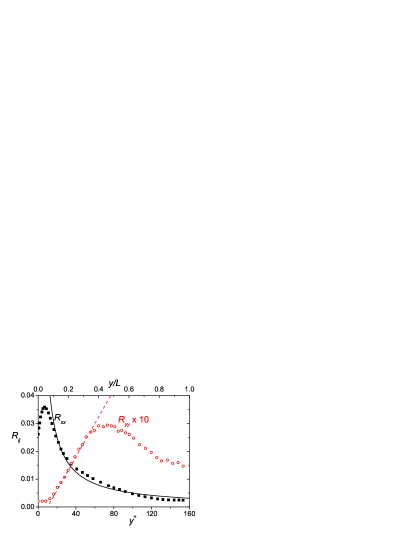
Figure 1: Comparison of the DNS data Ref. DNS2 for the mean profiles of the $xx$ and $yy$ components of the elastic stress tensor $\Pi_{0}^{ij}$ with analytical predictions. Black squares: DNS data for streamwise diagonal component $\Pi_{0}^{xx}$, that according to our understanding, Eq. (V.2), has to decrease as $1/y$ with the distance to the wall. Black solid line: $1/y^{+}$ dependence. Red empty circles: DNS data for the wall-normal component $\Pi_{0}^{yy}$, for which we predicted linear increase with $y^{+}$ in the log-law turbulent region. Red dashed line - linear dependence, $\propto y^{+}$.

The effective polymeric viscosity was measured, for example, in Ref. DNS1 , Fig. 5, and in Ref. Beta . In these Refs. $\nu_{\rm{p}}(y)$ was understood as $\Delta_{\rm{p}}(y)/S_{0}(y)$, where $\Delta_{\rm{p}}(y)$ is the Reynolds stress deficit, which is $\Pi_{0}^{xy}$ according to Eq. (10). The observations of Refs. DNS1 ; Beta is that $\nu_{\rm{p}}(y)$ in the turbulent boundary layer grows linearly with the distance from the wall. Recent data of DNS of the Navier-Stokes equation with polymeric additives (using the FENE-P model) taken from Ref. DNS2 are presented in Fig. 1. The wall-normal component $\Pi_{0}^{yy}$ is presented by the red empty circles. One sees that (in the quite narrow) region $20<y^{+}<60$ (where the mean velocity profile is close of MDR) the profile $\Pi_{0}^{yy}$ is indeed proportional to $y^{+}$, as represented by the red dashed line. This is in agreement with our result, see Eq. (57b) and our Ref. 03LPPT .

Direct DNS of other components of the polymeric stress tensor, see, e.g. Fig. 6 in Ref. DNS2 also agrees with the tensorial structure of $\bm{\Pi}_{0}$ given by Eq. (V.2).

VI Summary and discussion

The aim of this paper was the analysis of the polymer stress tensor in turbulent flows of dilute polymeric solutions. On the face of it this object is very hard to pinpoint analytically, being sensitive to complex interactions between the polymer molecules and the turbulent motions. We showed nevertheless that in the limit of very high Deborah numbers, ${{\mathcal{D}}}\mkern-3.1mue\gg 1$, this tensor attains a universal form. Increasing the complexity of our turbulent ensemble, from laminar, through homogeneous turbulence with a constant shear, and ending up with wall bounded anisotropic turbulence, we proposed a universal form

$$\bm{\Pi}_{0}(y)\simeq\Pi^{yy}_{0}(y)\left(\begin{array}[]{ccc}2{{\mathcal{D}}}\mkern-3.1mue^{2}(y)&~{}{{\mathcal{D}}}\mkern-3.1mue(y){}&~{}~{}0{}{}\\ {{\mathcal{D}}}\mkern-3.1mue(y)&1&0\\ 0&0&C(y)\end{array}\right)\ .$$ (61)

We rewrite this form here to stress that it remains unchanged even when the Deborah number, and with it the components of the tensor, become space dependent. Obviously, this strong result is expected to hold only as long as the mean properties, including the mean shear, vary in space in a controlled fashion, as for example in the logarithmic layer near the wall (be it a Kármán or a Virk logarithm).

As an important application of these results we considered in Sect. V the important problem of drag reduction by polymers in wall bounded flows. A difficult issue that caused a substantial confusion is the relation between the polymer physics, the effective viscosity that is due to polymer stretching, and drag reduction. In recent work on drag reduction it was shown that the Virk logarithmic Maximum Drag Reduction asymptote is consistent with a linearly increasing (with $y$) effective viscosity due to polymer stretching. This result seemed counter intuitive since numerical simulations indicated that polymer stretching is decreasing as a function of $y$. The present results provide a complete understanding of this conundrum. “Polymer stretching” is dominated by $\Pi_{0}^{xx}$ since it is much larger than all the other components of the stress tensor. As shown above, this component is indeed decreasing when $y$ increases, cf. Fig. 1. On the other hand the effective viscosity is proportional $\Pi_{0}^{yy}$, and this component is indeed increasing (linearly) with $y$, cf. Fig. 1. In fact, drag reduction saturates precisely when $\Pi_{0}^{xx}$ and $\Pi_{0}^{yy}$ become of the same order.

Appendix A Exact energy balance equations

In this Appendix we present exact energy balance equations that are useful in the analysis of turbulence of the polymeric solutions. In the present study we employ only one of them, i.e. Eq. (64e).

Introduce the mean densities of the turbulent kinetic energy $E_{\scriptscriptstyle\rm{T}}$ and polymeric potential energy $E_{\rm{p}}$

$$E_{\scriptscriptstyle\rm{T}} \equiv \frac{1}{2}W\,,\quad W\equiv\text{Tr}\,\{{\bm{W}}\}\,,$$ (62a)

$$E_{\rm{p}} \equiv \frac{1}{2}\Pi_{0}\,,\quad\Pi_{0}\equiv{\rm Tr}\,\{\bm{\Pi}_{0}\}\ .$$ (62b)

Using Eqs. (3) one can derive equations for the balance of $E_{\scriptscriptstyle\rm{T}}$ and $E_{\rm{p}}$ and for their sum:

$$\frac{DE_{\scriptscriptstyle\rm{T}}}{Dt} = \varepsilon^{+}_{\scriptscriptstyle\rm{T}}-\varepsilon^{-}_{\scriptscriptstyle\rm{T}}-{\varepsilon_{\scriptscriptstyle\rm{T}}}_{\rm{p}}=0\,,$$ (63a)

$$\frac{DE_{\rm{p}}}{Dt} = \varepsilon^{+}_{\rm{p}}-\varepsilon^{-}_{\rm{p}}+{\varepsilon_{\scriptscriptstyle\rm{T}}}_{\rm{p}}=0\,,$$ (63b)

$$\hskip-28.45274pt\frac{D}{Dt}\left(E_{\scriptscriptstyle\rm{T}}+E_{\rm{p}}\right) = \varepsilon^{+}_{\scriptscriptstyle\rm{T}}+\varepsilon^{+}_{\rm{p}}-\varepsilon^{-}_{\scriptscriptstyle\rm{T}}-\varepsilon^{-}_{\rm{p}}=0\ .$$ (63c)

We denote by $$\varepsilon^{+}_{\scriptscriptstyle\rm{T}} \varepsilon^{+}_{\rm{p}}$$ and the energy flux from the mean flow to the turbulent and polymeric subsystem respectively:

$$\varepsilon^{+}_{\scriptscriptstyle\rm{T}} \equiv -S_{0}W^{xy}\,,$$ (64a)

$$\varepsilon^{+}_{\rm{p}} \equiv S_{0}\Pi_{0}^{xy}\,;$$ (64b)

$$\varepsilon^{-}_{\scriptscriptstyle\rm{T}} \varepsilon^{-}_{\rm{p}}$$ describes the dissipation of energy in the turbulent subsystem, whereas is the dissipation in the polymeric subsystem due to the relaxation of the stretched polymers back to equilibrium:

$$\varepsilon^{-}_{\scriptscriptstyle\rm{T}} \equiv \nu_{0}\text{Tr}\left\langle\bm{s}\cdot\bm{s}^{\scriptscriptstyle\rm{T}}\right\rangle\,,$$ (64c)

$$\varepsilon^{-}_{\rm{p}} \equiv \frac{1}{2\,\tau_{\rm{p}}}{\rm Tr}\left(\bm{\Pi}_{0}-\bm{\Pi}_{\rm{eq}}\right)\ .$$ (64d)

The last term on the RHS of Eqs. (63a) and (63b) [that is absent in (63c)] describes the energy exchange between the polymeric and turbulent subsystems:

$${\varepsilon_{\scriptscriptstyle\rm{T}}}_{\rm{p}}\equiv\text{Tr}\left\langle\bm{s}\cdot{\bm{\pi}}\right\rangle=\frac{1}{2}{\rm Tr}\,\{\bm{Q}_{\scriptscriptstyle\rm{T}}\}\ .$$ (64e)

Using the expression for the momentum flux, we obtain an exact balance equation for the total energy

$$E=E_{\scriptscriptstyle\rm{V}}+E_{\scriptscriptstyle\rm{T}}+E_{\rm{p}}\,,$$ (65a)

that in the stationary state reads:

$$S_{0}{\cal P}=\frac{1}{2\tau_{\rm{p}}}{\rm Tr}\left(\bm{\Pi}_{0}-\bm{\Pi}_{\rm{eq}}\right)+\nu_{0}\left(S_{0}^{2}+{\rm Tr}\left\langle\bm{s}\cdot\bm{s}^{\scriptscriptstyle{\rm T}}\right\rangle\right)\,.$$ (65b)

In Eq. (65a) $E_{\scriptscriptstyle\rm{V}}$ is the density of the kinetic energy of the mean flow, defined up to an arbitrary constant, depending on the choice of the origin of coordinates. The LHS of Eq. (65b) describes the work of external forces needed to maintain the constant mean shear. The first term on the RHS ($\propto{1}/{\tau_{\rm{p}}}$) describes the energy dissipation in the polymeric subsystem. The term $\nu_{0}S_{0}^{2}$ represents the viscous dissipation due to the mean shear, while the last term on the RHS is responsible for the viscous dissipation caused by the turbulent fluctuations.

References

• (1) B.A. Toms, in Proceedings of the International Congress of Rheology Amsterdam Vol 2. 0.135-141 (North Holland, 1949).
• (2) P.S. Virk, AIChE J. 21, 625 (1975).
• (3) P.G. de Gennes, Introduction to Polymer Dynamics, (Cambridge, 1990).
• (4) K. R. Sreenivasan and C. M. White, J. Fluid Mech. 409, 149 (2000).
• (5) J.L. Lumley, Annu. Rev. Fluid Mech. 1, 367 (1969).
• (6) J.L. Lumley, Symp. Math 9, 315 (1972).
• (7) M. Tabor and P.G. de Gennes, Europhys. Lett. 2, 519 (1986).
• (8) E. Balkovsky, A. Fouxon, and V. Lebedev, ”Turbulent Dynamics of Polymer Solutions”, Phys. Rev. Lett. 84, 4765 (2000).
• (9) E. Balkovsky, A. Fouxon, and V. Lebedev,, ”Turbulence of polymer solutions” Phys. Rev. E 64, 056301 (2001).
• (10) M. Chertkov, ”Polymer Stretching by Turbulence”, Phys. Rev. Lett. 84, 4761 (2000).
• (11) V.S. L’vov, A. Pomyalov, I. Procaccia and V. Tiberkevich, Phys. Rev. Lett., in press. Also: nlin.CD/0307034
• (12) K. Furutsu, J. Res. NBSD 67, 303, (1963)
• (13) A.E. Novikov, Soviet Physics, JETP, 47, 1919 (1964).
• (14) T. Burghelea, V. Steinberg and P.H. Diamond, Europhys. Lett. 60, 704, (2002).
• (15) R. benzi, E. de Angelis, V.S. L’vov, I. Procaccia and V. Tiberkevich, β€œMaximum Drag Reduction Asymptotes and the Cross-Over to the Newtonian Plug”, J. Fluid Mech, submitted.
• (16) R. Sureshkuar and A.N. Beris, Phys. of Fluids, 9, 743, (1997).
• (17) E. de Angelis, PhD thesis, Univ. di Roma β€œLa Saspienza” (2000).
• (18) E. de Angelis, C.M. Casciola and R. Piva, CFD Journal, 9, 1 (2000).
• (19) S. Sibilla and A. Baron, Phys. of Fluids, 14, 1123 (2002).
• (20) P. K. Ptasinski et. al, J. Fluid Mech., 490, 251 (2003).