Understanding Anomalous Transport in Intermittent Maps:
From Continuous Time Random Walks to Fractals

Abstract

We show that the generalized diffusion coefficient of a subdiffusive intermittent map is a fractal function of control parameters. A modified continuous time random walk theory yields its coarse functional form and correctly describes a dynamical phase transition from normal to anomalous diffusion marked by strong suppression of diffusion. Similarly, the probability density of moving particles is governed by a time-fractional diffusion equation on coarse scales while exhibiting a specific fine structure. Approximations beyond stochastic theory are derived from a generalized Taylor-Green-Kubo formula.

The notion of anomalous diffusion derives from the fact that the mean squared displacement (MSD) must not follow the law of normal diffusion, $<x^{2}>\sim t^{\gamma}$ with $\gamma=1$, but may be superdiffusive with $\gamma>1$ or subdiffusive with $\gamma<1$. Such anomalous dynamics has been investigated theoretically and observed experimentally not only in amorphous semiconductors, surface diffusion, turbulence, polymers and plasmas but also in chemical, biological and economical problems Bou90 ; Met00 . For this variety of applications it is desirable to have a class of test systems at hand which are yet easy to handle. Here periodically continued deterministic maps provide an important basis for analytical and numerical investigations Gei84 ; Gei85 ; Zum93 ; Zum93a ; Sto95 ; Bar03 . Both the sub- and the superdiffusive dynamics of such models was successfully described by continuous time random walk (CTRW) approaches Gei84 ; Zum93 ; Zum93a ; Bar03 . This stochastic theory yields non-Gaussian probability density functions (PDF) for anomalous diffusive processes exhibiting stretched exponential decay in case of sub- and Lévy power law decay in case of superdiffusion Zum93 .

On the other hand, a microscopic theory of anomalous deterministic transport explaining the origin of this behavior in terms of the theory of dynamical systems is just beginning to evolve Sto95 . Surprises along these lines were already encountered in normal diffusive maps, where the diffusion coefficient was found to be a fractal function of control parameters Kla95 ; Kla96 . This behavior was also reported for more complex systems like the climbing sine map Kor02 , bouncing ball billiards Har01 and coupled Josephson junctions Tan02 . The fractality can be understood as a signature of long-range dynamical correlations that, due to topological instabilities, change in a complicated manner under parameter variation Kla02 . However, no such fractal structures were yet identified in anomalous dynamics as modeled by the maps of Refs. Gei84 ; Gei85 ; Zum93 ; Zum93a ; Sto95 ; Bar03 .

In this Letter we focus on a subdiffusive map whose functional form on the unit interval was introduced by Pomeau and Manneville for describing intermittency Pom80 ,

$$x_{n+1}\equiv M_{a,z}(x_{n})=x_{n}+ax_{n}^{z},\;\;0\leq x_{n}<\frac{1}{2}.$$ (1)

For $\frac{1}{2}\leq x_{n}<1$ the map is defined according to $M_{a,z}(-x)=-M_{a,z}(x)$. The translation $M_{a,z}(x+m)=M_{a,z}(x)+m$, $m\in\mathbb{Z}$, completes the definition on the real line, see the inset of Fig. 1 (a). The degree of nonlinearity $z\geq 1$ and $a\geq 1$ in Eq. (1) hold for the two control parameters. For $1\leq z<2$ this model leads to normal diffusion while for $z\geq 2$ its behavior is anomalous Gei84 ; Zum93 . The anomalous regime results from the existence of marginal fixed points located at all integer values of $x$. Thus, a typical trajectory of the map consists of long laminar phases interrupted by chaotic bursts. In contrast to Refs. Gei84 ; Zum93 , which focused on the time dependence of the MSD for the particular parameter value of $a=2^{z}$, here we study the behavior of the generalized diffusion coefficient (GDC) Met00

$$K:=\lim_{n\rightarrow\infty}\frac{\left<x^{2}\right>}{n^{\gamma}}\>$$ (2)

($<\ldots>$ denotes an ensemble average) for this map under variation of both control parameters. We first focus on numerical simulations sim of the map Eq. (1) and on the interpretation of the results within the CTRW approach. CTRW theory models diffusion processes by sequences of jumps interrupted by periods of waiting. Let the PDFs of waiting times and of jump lengths be defined by $\phi(t)$ and $\lambda(x)$, respectively. Choosing these functions appropriately, CTRW theory predicts that $\gamma=1$ for $1\leq z<2$ and $\gamma=1/(z-1)$ for $2<z$ irrespective of the parameter $a$ of the map Gei84 ; Zum93 . Indeed, for all $a$ we find excellent agreement between these solutions and the values for $\gamma$ obtained from simulations. Consequently, the analytical expressions for $\gamma$ are used throughout our work.

Simulation results for $K$ as a function of $a$ for fixed $z$ are presented in Fig. 1. Magnifications of Fig. 1 (a) shown in parts (b) and (c) reveal self similar-like irregularities indicating a fractal parameter dependence of $K$. Note particularly the structure marked by triangles, which is repeated on finer and finer scales. The parameter values for these symbols correspond to specific series of Markov partitions Kla95 ; Kla96 . In Fig. 2 $K$ is depicted as a function of $z$ for different values of $a$, again displaying highly non-monotonic parameter dependences.

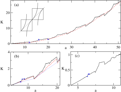
Figure 1: The generalized diffusion coefficient $K$, Eq. (2), as a function of $a$ for $z=3$. The curve in (a) consists of $1200$ points, the dashed-dotted line displays the CTRW result $K_{1}$, Eqs. (5), (7). (b) (600 points) and (c) (200 points) show magnifications of (a) close to the onset of diffusion. The dotted line in (b) is the CTRW approximation $K_{2}$, Eqs. (6), (7). The dashed line represents the first term of the TGK formula Eq. (8). The triangles mark a specific structure appearing on finer and finer scales. The inset depicts the model Eq. (1). All quantities here and in the following figures are dimensionless.

In a first step for explaining these curves we apply standard CTRW theory Gei84 ; Zum93 by modifying this approach at three points: Firstly, the waiting time PDF must be calculated according to the grid of elementary cells indicated in Fig. 1 Kla96 ; Kla97 yielding

$$\phi(t)=a\left(1+a(z-1)t\right)^{-\frac{z}{z-1}}\>.$$ (3)

Secondly, as a jump probability we use

$$\lambda(x)=\frac{p}{2}\delta(\left|x\right|-l)+(1-p)\delta(x)\>.$$ (4)

The second term accounts for the fact that particles may stay in a box with a probability of $(1-p)$. This quantity is roughly determined by the size of the escape region $p=(1-2x_{c})$ with $x_{c}$ as a solution of the equation $x_{c}+ax^{z}_{c}=1$. Thirdly, we introduce two definitions of a typical jump length $l_{i}\>,i\in\{1,2\}$. Thus,

$$l_{1}=\left\{|M_{a,z}(x)-x|\right\}\>$$ (5)

corresponds to the actual mean displacement while

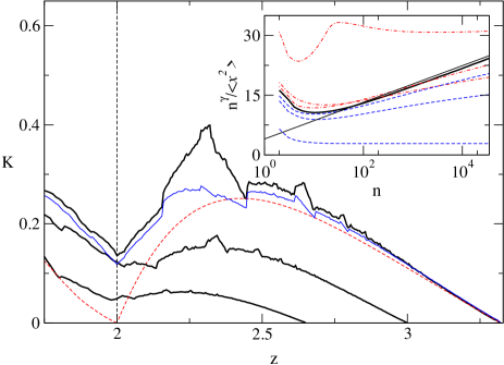
Figure 2: $K$ as a function of $z$ for $a=3.14,4,5$ consisting of $200$, $250$ and $300$ points (bottom to top). Bold lines represent simulation results for $n=10^{4}$ iterations, the dashed line is the CTRW solution $K_{2}$, Eqs. (6), (7), for $n\to\infty$. The thin line displays the first term of the TGK formula Eq. (8). At $z=2$ there is a transition from normal to anomalous diffusion. The inset describes the time-dependence of $<x^{2}>$ around this value with $a=3.14$. Here dashed lines correspond to $z=1.5,1.9,1.95$ (bottom to top), dashed-dotted lines to $2.5,2.1,2.05$ (top to bottom) while the bold line depicts $z=2$. The dotted line is proportional to $\ln(n)$.

$$l_{2}=\left\{|[M_{a,z}(x)]|\right\}\>$$ (6)

gives the coarse-grained displacement in units of elementary cells, as it is often assumed in CTRW approaches. In these definitions $\left\{\ldots\right\}$ denotes both a time and ensemble average over particles leaving a box. The modified CTRW approximation for the GDC resulting from these three changes reads

$$K_{i}=\begin{cases}pl_{i}^{2}a^{\gamma}\sin(\pi\gamma)/\pi\gamma^{1+\gamma},&0<\gamma<1\cr pl_{i}^{2}a(1-1/\gamma),&1\leq\gamma<\infty\>.\end{cases}$$ (7)

Fig. 1 (a) shows that $K_{1}$ well describes the coarse functional form of $K$ for large $a$. $K_{2}$ is depicted in Fig. 1 (b) by the dotted line and is asymptotically exact in the limit of $a\to 0$. Hence, the GDC exhibits a dynamical crossover analogous to the one found for normal diffusion Kla96 ; Kla97 ; Kor02 . Let us now focus on the GDC at $a=12,20,28,...$, which corresponds to integer values of the height $h=[M_{a,z}(1/2)]$ of the map. Simulations reproduce, within numerical accuracy, the results for $K_{2}$ by indicating that $K$ is discontinuous at these parameter values. Due to the self similar-like structure of the GDC we arrive at the conjecture that $K$ exhibits infinitely many discontinuities on fine scales as a function of $a$, in contrast to the continuity of the CTRW solution.

We now switch back to the $z$-dependence of $K$, where CTRW theory predicts a dynamical phase transition from normal to anomalous diffusion at $z=2$ Gei84 ; Zum93 . At the transition point one has $<x^{2}>\sim n/\log(n)$. According to Eq. (2), Eq. (7) yields a continuous transition in $z$, see $K_{2}$ in Fig. 2. However, this coarse functional form is obscured not only by fractal irregularities but also by an ultra-slow convergence of the MSD in our simulations. Using CTRW theory, we verified that around $z=2$ the MSD is determined by a series of logarithmic corrections in time, where the lowest-order term is proportional to $n^{\gamma}/\log n$ and dominates at time scales controlled by $n\ll\tilde{n}\sim\exp(1/(1-\gamma))$. Hence, for $\gamma\neq 1$ and $n\gg\tilde{n}$ simple power laws are recovered while for $\gamma=1$ this logarithmic term survives in the infinite time limit. The inset of Fig. 2 exemplifies this behavior explaining deviations between CTRW theory and the simulation results in the main figure. In other words, around $z=2$ both normal and anomalous diffusion are suppressed due to logarithmic corrections in time leading to a vanishing $K$. We strongly suspect that such a behavior of the GDC is typical for dynamical phase transitions in anomalous dynamics altogether Zum93a .

The stochastic CTRW theory presented above describes only the coarse parameter dependence of the GDC. This motivates us to develop an approach that incorporates dynamical correlations. For this purpose we generalize the Taylor-Green-Kubo formula (TGK) Remark2 for maps to anomalous diffusion. We start by expressing Eq. (2) via sums over the integer velocities $v_{m}=\left[x_{m+1}\right]-\left[x_{m}\right]$ Kla02 . However, in contrast to normal diffusion the anomalous dynamics generated by Eq. (1) is not stationary for $z\geq 2$ Gas88 ; Zum93a . This is reminiscent in the non-existence of an invariant probability density for this map, or mathematically, in the existence of infinite invariant measures Aar . Consequently, the resulting expression cannot be simplified using time-translational invariance, and we get

$$K=\lim_{n\rightarrow\infty}\frac{1}{n^{\gamma}}\left[<\sum_{k=0}^{n-1}v_{k}^{2}>+2<\sum_{k=0}^{n-1}\sum_{l=1}^{n-1}v_{k}v_{k+l}>\right]\>.$$ (8)

Focusing on the first term only, simulations confirm that it is proportional to $n^{\gamma}$. For $z<2$ the dynamics is ergodic, hence this term is equal to $n<v_{0}^{2}>$, and we recover the random walk formula for normal diffusion Kla96 ; Kla97 . For $z\geq 2$ only generalized ergodic theorems may hold Aar , and whether the CTRW result Eq. (7) can be derived from the first term is a non-trivial question. Considering this term as an approximation of $K$ for all $z$, the numerical results are depicted in Figs. 1 (b) and 2. The comparison of this data with the simulation values based on Eq. (2) indeed shows that this term already provides a first step beyond the modified CTRW model: In the $a$ dependence it reproduces the major irregularities of $K$ and even appears to follow the discontinuities discussed above. However, we cannot say yet whether it yields exact values for $K$ at integer heights.

Eq. (8) thus provides a suitable starting point for a systematic understanding of the fractal GDC beyond CTRW theory. We remark that already the first term can be related to de Rham-type fractal functions, which explains why it features irregularities Unp . Since the series expansion in Eq. (8) is exact, working out further terms one must recover more and more structure in the GDC Kla96 ; Kla02 ; Kor02 . Note that the correlation function in the second term depends on two times, which enables to express $K$ in terms of aged Bar03 de Rham-type fractal functions summing up to the exact value.

Figure 3: Comparison of the PDF obtained from simulations of the map Eq. (1) (oscillatory structure) with the analytical solution Eq. (10) of the fractional diffusion equation Eq. (9) (continuous line in the middle) for $z=3$ and $a=8$. The PDF was computed from $10^{7}$ particles after $n=10^{3}$ iterations. For the GDC in Eq. (10) the simulation result was used. The crosses (x) represent the numerical results coarse grained over unit intervals. The upper and the lower curves correspond to fits with a stretched exponential and a Gaussian distribution, respectively. The inset depicts the PDF for the map on the unit interval with periodic boundaries.

We now turn to the PDFs generated by the map Eq. (1). The great success of CTRW theory derives from the fact that it correctly predicts both the power $\gamma$ and the form of the coarse grained PDF $P(x,t)$ of displacements for a large class of models Zum93 . Correspondingly, the diffusion process generated by Eq. (1) is not described by an ordinary diffusion equation but by a fractional generalization of it. Starting from the CTRW model for the map Eq. (1) discussed above, one can derive the time-fractional diffusion equation

$$\frac{\partial^{\gamma}P(x,t)}{\partial t^{\gamma}}\equiv\int_{0}^{t}dt^{{}^{\prime}}(t-t^{{}^{\prime}})^{-\gamma}\frac{\partial P}{\partial t^{{}^{\prime}}}=D\frac{\partial^{2}P}{\partial x^{2}}$$ (9)

describing the long-time limit of the PDF of the coarse grained dynamics with initial condition $P(x,0)=\delta(x)$ and $D=K\Gamma(1+\gamma)/2$, $0<\gamma<1$. The fractional derivative is understood in the Caputo sense Mai97 . Time-fractional equations of such a form have already been extensively studied by mathematicians Gor00 . We remark that the two other fractional diffusion equations proposed in Refs. Bar03 ; Met00 , which are based on a Riemann-Liouville fractional derivative, are equivalent to Eq. (9) under rather weak assumptions ACunp . The solution of Eq. (9) expressed in terms of an M-function of Wright type Mai97 ; Gor00 reads

$$P(x,t)=\frac{1}{2\sqrt{D}t^{\gamma/2}}M\left(\xi,\frac{\gamma}{2}\right)$$ (10)

giving exactly the same asymptotics that was obtained in Ref. Zum93 for small and large values of $\xi=|x|/\sqrt{D}t^{\gamma/2}$. By using a series representation of $M$ it can be demonstrated ACunp that this form is equivalent to those expressed via H-functions Met00 or one-sided extremal Lévy stable distributions Bar03 . Fig. 3 demonstrates an excellent agreement between the analytical solution Eq. (10) and the PDF obtained from simulations for the map Eq. (1) if the PDF is coarse grained over unit intervals. However, it also shows that the coarse graining eliminates a periodic fine structure that is not captured by Eq. (10) Kla96 . This fine structure derives from the ‘microscopic’ PDF of an elementary cell (with periodic boundaries) as represented in the inset of Fig. 3. The singularities are due to the marginal fixed points of the map, where particles are trapped for long times. Remarkably, that way the microscopic origin of the intermittent dynamics is reflected in the shape of the PDF on the whole real line: From Fig. 3 it is seen that the oscillations in the PDF are bounded by two functions, the upper curve being of a stretched exponential type while the lower is Gaussian. These two envelopes correspond to the laminar and chaotic parts of the motion, respectively Remark3 .

In conclusion, we have shown that the anomalous dynamics generated by a paradigmatic subdiffusive one-dimensional map exhibits a fractal GDC under variation of control parameters. The coarse dependence of this GDC and a non-trivial phase transition from normal to anomalous diffusion are captured by a modified CTRW theory. Near the phase transition point the GDC is strongly suppressed by logarithmic corrections in time. A more detailed understanding of the GDC is provided by an anomalous TGK formula suggesting intimate relations to aging, fractal functions and ergodic theory. The coarse-grained PDF of this anomalous dynamics is in excellent agreement with the solution of a suitable fractional diffusion equation while on fine scales it reflects the microscopic details of the intermittent dynamics. Here we have only treated a subdiffusive map, however, we expect these findings to be typical for spatially extended, low-dimensional, anomalous deterministic dynamical systems altogether. Further studies will focus on a more detailed analysis of the anomalous TGK-formula, on a spectral analysis of this map and on treating superdiffusive dynamics along the same lines.

The authors acknowledge helpful discussions with J. Klafter, R. Metzler and A. Pikovsky. They thank the MPIPKS Dresden for hospitality and financial support. IMS acknowledges partial financial support by the Fonds der Chemischen Industrie.

References

- (1) J.-P. Bouchaud, A. Georges, Phys. Rep. 195, 127 (1990); M.F. Shlesinger, G.M. Zaslavsky, and J. Klafter, Nature (London) 263, 31 (1993); J. Klafter, M.F. Shlesinger, G. Zumofen, Phys. Today 49, 32 (1996); I.M. Sokolov, J. Klafter, A. Blumen, Phys. Today 55, 48 (2002).
- (2) R. Metzler, J. Klafter, Phys. Rep. 339, 1 (2000).
- (3) T. Geisel, S. Thomae, Phys. Rev. Lett. 52, 1936 (1984).
- (4) T. Geisel, J. Nierwetberg, A. Zacherl, Phys. Rev. Lett. 54, 616 (1985).
- (5) G. Zumofen, J. Klafter, Phys. Rev. E 47, 851 (1993).
- (6) G. Zumofen, J. Klafter, Physica D 69, 436 (1993).
- (7) R. Stoop, Phys. Rev. E 52, 2216 (1995); C. Dettmann, P. Cvitanovic, Phys. Rev. E 56, 6687 (1997); Tasaki, P. Gaspard, Physica D 187, 51 (2004); R. Artuso, G. Cristadoro, Phys. Rev. Lett. 90, 244101 (2003).
- (8) E. Barkai, Phys. Rev. Lett. 90, 104101 (2003).
- (9) R. Klages, J.R. Dorfman, Phys. Rev. Lett. 74, 387 (1995); Phys. Rev. E 59, 5361 (1999).
- (10) R. Klages, Deterministic Diffusion in One-Dimensional Chaotic Dynamical Systems (Wissenschaft & Technik Verlag, Berlin, 1996).
- (11) N. Korabel, R. Klages, Phys. Rev. Lett. 89, 214102 (2002); Physica D 187, 66 (2004).
- (12) T. Harayama, P. Gaspard, Phys. Rev. E 64, 036215 (2001); L. Matyas, R. Klages, Physica D 187, 165 (2004).
- (13) K.I. Tanimoto, T. Kato, and K. Nakamura, Phys. Rev. B 66, 012507 (2002).
- (14) R. Klages N. Korabel, J. Phys. A: Math. Gen. 35, 4823 (2002).
- (15) Y. Pomeau, P. Manneville, Commun. Math. Phys. 74, 189 (1980); P. Manneville, J. Physique 41, 1235 (1980)
- (16) All simulations were performed starting from a uniform, random distribution of initial conditions on the unit interval by iterating for time steps.
- (17) R. Klages, J.R. Dorfman, Phys. Rev. E 55, R1247 (1997).
- (18) The so-called Green-Kubo formula for diffusion was already derived in G.I. Taylor, Proc. Lond. Math Soc. 20, 196 (1921).
- (19) P. Gaspard, X.-J. Wang, Proc. Natl. Acad. Sci. 85, 4591 (1988).
- (20) J. Aaronson, LMS lecture notes 277, 1 (2000); H. Hu, L.-S. Young, Erg. Th. Dyn. Syst. 15, 67 (1995).
- (21) N. Korabel et al., in preparation.
- (22) F. Mainardi, Fractional Calculus: Some Basic Problems in Continuum and Statistical Mechanics. in: A. Carpinteri and F. Mainardi (Eds.), Fractals and Fractional Calculus in Continuum Mechanics, p.291 (Springer, New York, 1997).
- (23) R. Gorenflo, Y, Luchko, F. Mainardi, J. Comp. Appl. Math. 118, 175 (2000).
- (24) I.M. Sokolov, A. Chechkin and J. Klafter, Acta Physica Polonica B, in press.
- (25) The two envelopes shown in Fig. 3 represent fits with the Gaussian and with the M-function , where , and , .