Introduction

As it is now widely recognized, classical dynamical chaos has been one of the major scientific breakthroughs of the past century. On the other hand, the manifestations of chaotic motion in quantum mechanics, though widely studied [1, 2], remain somehow not so clearly understood, both from the mathematical as well as from the physical point of view.

The difficulty in understanding chaotic motion in terms of quantum mechanics is rooted in two basic properties of quantum dynamics:

1. The energy spectrum of bounded, finite number of particles, conservative quantum systems is discrete. This means that the quantum motion is ultimately quasi-periodic, i.e. any temporal behaviour is a discrete superposition of finitely or countably many Fourier components with discrete frequencies. In the ergodic theory of classical dynamical systems, such a quasi-periodic dynamics corresponds to the limiting case of integrable or ordered motion while chaotic motion requires continuous Fourier spectrum [3].

2. Quantum motion is dynamically stable, i.e. initial errors propagate only linearly with time [4]. Linear instability is a typical feature of classical integrable systems and this contrasts the exponential instability which characterizes classical chaotic systems.

Therefore it appears that quantum motion always exhibits the characteristic features of classical integrable, regular motion which is just the opposite of dynamical chaos. However, it has been shown that this apparently paradoxical situation can be resolved with the introduction of different time scales inside which the typical features of classical chaos are present in the quantum motion also. Since these time scales diverge as Planck constant $\hbar$ goes to zero, no contradiction arises with the correspondence principle [5].

Still the state of affairs remains unsatisfactory. For example one should build a statistical theory for systems with discrete spectrum and linear instability. In this connection the question whether, in order to have the quantum to classical transition, external noise (or coupling to external macroscopic number of degrees of freedom) is necessary or not, remains unclear. Indeed it is generally accepted that external noise may induce the non-unitary evolution leading to the decay of non-diagonal matrix elements of the density matrix in the eigenbasis of the physical observables, thus restoring the classical behaviour. On the other hand it has also been surmised that external noise, being sufficient, is not necessary. A new type of decoherence – the dynamical decoherence– has been proposed [5], without any noise and only due to the intrinsic chaotic evolution of a pure quantum state. The simplest manifestations of dynamical decoherence are the fluctuations in the quantum steady state which, in the quasi-classical region, is a superposition of very many eigenfunctions. In case of a quantum chaotic - ergodic steady state - all eigenfunctions essentially contribute to the fluctuations and their contribution is statistically independent[5]. This fact suggests the complete quantum decoherence in the final steady state for any initial state even though the steady state is formally a pure quantum state. Yet this argument is not completely convincing and a more clear evidence is required. In this letter we discuss this question by considering one of the basic experiments on which rests quantum mechanics, namely a phenomenon which, in the words of Richard Feynmann [6], ”… is impossible absolutely impossible, to explain in any classical way, and which has in it the heart of quantum mechanics. In reality, it contains the only mystery.” : the double slit experiment.

Experiment

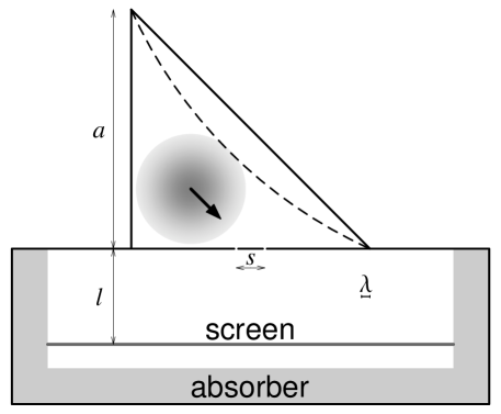
Figure 1: The geometry of the numerical double-slit experiment. All scales are in proper proportions. The two slits are placed at a distance $s$ on the lower side of the billiard

We have performed the following numerical, double-slit experiment. The time dependent Schrödinger equation ${\rm i}\hbar\frac{\partial}{\partial t}\Psi(x,y,t)={\hat{H}}\Psi(x,y,t)$, with ${\hat{H}}={\hat{p}}^{2}/(2m)$, has been solved numerically (see Method section) for a quantum particle which moves freely inside the two-dimensional domain as indicated in fig. 1 (full line). Note that the domain is composed of two regions which are connected only through two narrow slits. We refer to the upper bounded region as to the billiard domain, and to the lower one as the radiating region. The scaled units have been used in which Planck’s constant $\hbar=1$, mass $m=1$, and the base of the triangular billiard has length $a=1$. The initial state $\Psi(t=0)$ is a Gaussian wave packet (coherent state) centered at a distance $a/4$ from the lower-left corner of the billiard (in both Cartesian directions) and with velocity $\vec{v}$ pointing to the middle between the slits. The screen is at a distance $l=0.4$ from the base of the triangle. The magnitude of velocity $v$ (in our units equal to the wave-number $k=v$) sets the de Broglie wavelength $\lambda=2\pi/k$. In our experiment we have chosen $k=180$ corresponding to approximately $1600$th excited states of the closed quantum billiard. The slits distance has been set to $s=0.1\approx 3\lambda$ and the width of the slits is $d=\lambda/4$. The wave-packet is also characterized by the position uncertainty $\sigma_{x}=\sigma_{y}=0.24$. This was chosen as large as possible in the present geometry in order to have a small uncertainty in momentum $\sigma_{k}=1/(2\sigma_{x})$.

The lower, radiating region, should in principle be infinite. Thus, in order to efficiently damp waves at finite boundaries, we have introduced an absorbing layer around the radiating region. More precisely, in the region referred to as absorber, we have added a negative imaginary potential to the Hamiltonian $H\to H-{\rm i}V(x,y),V\geq 0$, which, according to the time dependent Schrödinger equation, ensures exponential damping in time. In order to minimize any possible reflections from the border of the absorber, we have chosen $V$ to be smooth, starting from zero and then growing quadratically inside the absorber. No significant reflection from the absorber was detected and this ensures that the results of our experiment are the same as would be for an infinite radiating region.

While the wave-function evolves with time, a small probability current leaks from the billiard and radiates through the slits. The radiating probability is recorded on a horizontal line $y=-l$ referred to as the screen. The experiment stops when the probability that the particle remains in the billiard region becomes vanishingly small. We define the intensity at the position $x$ on the screen as the perpendicular component of the probability current, integrated in time

$$I(x)=\int_{0}^{\infty}\!\!{\rm d}t\,{\rm Im}\,\Psi^{*}(x,y,t)\frac{\partial}{\partial y}\Psi(x,y,t)|_{y=-l}.$$ (1)

By conservation of probability the intensity is normalized, $\int_{-\infty}^{\infty}{\rm d}xI(x)=1$, and is positive $I(x)\geq 0$. $I(x)$ is interpreted as the probability density for a particle to arrive at the screen position $x$. According to the usual double slit experiment with plane waves, the intensity $I(x)$ should display interference fringes when both slits are open, and would be a simple unimodal distribution when only a single slit is open. This is what we wanted to test with a more realistic, confined geometry. The resulting intensities are shown in figs. 2, 3(red curves).

Indeed, a very clear (symmetric) interference pattern was found, with a visibility of the fringes depending on the parameters of the initial wave-packet. This can be heuristically understood as a result of integrability of the corresponding billiard dynamics. Namely, the classical ray dynamics inside a $\pi/4$ right triangular billiard is regular representing a completely integrable system. We know that each orbit of an integrable system is characterized by the fact that, since the classical motion in $2N$ dimensional phase space is confined onto an $N$ invariant torus, at each point in position space, e.g. at the positions of the slits, only a finite number of different momenta (directions) are possible. Thus the quantum wave-function, in the semiclassical regime, is expected to be locally a superposition of finitely many plane-waves[8] and the interference pattern on the screen is expected to be simply a superposition of fringes using these plane waves. In our case of an integrable $\pi/4$ right triangular billiard, different directions result from specular reflections with the walls. In contrast to the idealized plane-wave experiment in infinite domain where interference pattern depends on the direction of the impact, the fringes here were always symmetric around the center of the screen. This is a consequence of the presence of the vertical billiard wall, namely due to collisions with this wall each impact direction $(v_{x},v_{y})$ is always accompanied with a reflected direction $(-v_{x},v_{y})$. The pattern on the screen is then a symmetric superposition of the two interference images, one being a reflection ($x\to-x$) of the other. In this way one can also understand that the visibility of the interference fringes may vary with the direction of the initial packet.

We also remark that the spacing between interference fringes is in agreement with the usual condition for plane waves that the difference of the distances from the two slits to a given point on the screen is an integer multiple of $\lambda$.

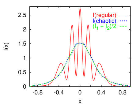
Figure 2: The total intensity after the double-slit experiment as a function of the position on the screen. $I(x)$ is obtained as the perpendicular component of the probability current, integrated in time. The red full curve indicates the case of regular billiard, while the blue dotted curve indicates the case of chaotic one. The green dashed curve indicates the averaged intensity over two 1-slit experiments, with either the regular or chaotic billiard (with results being practically the same, see fig. 3).

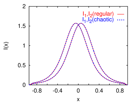
Figure 3: The two pairs of curves represent the intensities on the screen for the two 1-slit experiments (with either one of the two slits closed). The red full curves indicate the case of the regular billiard while the blue dotted ones indicate the case of chaotic billiard.

Now we make a simple modification of our experiment. We replace the hypotenuse of the triangle by the circular arc of radius $R=2$ (dashed curve in fig. 1). This change has a dramatic consequence for the classical ray dynamics inside the billiard, namely the latter becomes fully chaotic. In fact such a dispersive classical billiard is rigorously known to be a $K$-system [3]. Quite surprisingly, this has also a dramatic effect on the result of the double slit experiment. The interference fringes almost completely disappear, and the intensity can be very accurately reproduced by the sum of intensities $(I_{1}(x)+I_{2}(x))/2$ for the two experiments where only a single slit is open. This means that the result of such experiment is the same as would be in terms of classical ray dynamics. Notice however, that at any given instant of time, there is a well definite phase relation between the wave function at both slits. Yet, as time proceeds, this phase relation changes, and it is lost after averaging over time. This is nicely illustrated by the snapshots of the wave-functions in the regular and chaotic case shown in fig. 4. While in the regular case, the jets of probability emerging from the slits always point in the same direction and produce a clear time-integrated fringe structure on the screen, in the chaotic case, the jets are trembling and moving left and right, thus upon time-integration they produce no fringes on the screen[7].

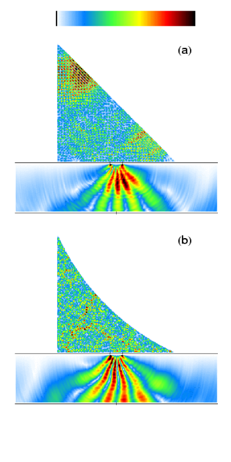
Figure 4: Typical snapshots of the wave-function (plotted is the probability density) for the two cases: (a) for the regular billiard at $t=0.325$, and (b) for the chaotic billiard at $t=0.275$ (both cases correspond to about half the Heisenberg time). The probability density is normalized separately in both parts of each plot, namely the probability density, in absolute units, in the radiating region is typically less than $1\%$ of the probability density in the billiard domain. The screen, its center, and the positions of the slits are indicated with thin black lines. Please note that the color code on the top of the figure is proportional to the square root of probability density.

Discussion and conclusions

The results of this numerical experiment can be understood in terms of fast decay of spatial correlations of eigenfunctions of chaotic systems. In the limit of small slits opening $d\ll\lambda$, the intensity on the screen, according to simple perturbation expansion in the small parameter $d/\lambda$, can be written as

$$I(x)=I_{1}(x)+I_{2}(x)+C(s)f(x),$$ (2)

where $f(x)$ is some oscillatory function determining the period of the fringes, and $C(s)$ is the spatial correlation function of the normal derivative of the eigenfunctions $\Psi_{n}$ of the closed billiard at the positions $(-s/2,0)$ and $(s/2,0)$ of the slits, written in the Cartesian frame with origin in the middle point between the slits. In particular, $C(s)=\alpha\sum_{n}|c_{n}|^{2}\partial_{y}\Psi_{n}(-s/2,0)\partial_{y}\Psi_{n}(s/2,0)$, where $c_{n}$ are the expansion coefficients of the initial wave-packet in the eigenstates $\Psi_{n}$, and $\alpha$ is a constant such that $C(0)=1$. Note that this eigenstate correlation function $C(s)$, which also depends on the initial state through the expansion coefficients $c_{n}$, is directly proportional to the visibility of the fringes. While it is known [8] that, for classically chaotic billiards, quantum eigenstates exhibit decaying correlations with $C(s)=J_{0}(ks)$ where $J_{0}$ is a zeroth order Bessel function, for regular systems $C(s)$ typically does not decay (but oscillates) so it produces interference fringes. In our case of half-square billiard we find, for large $k$, $C(s)=e^{-\sigma_{k}^{2}s^{2}/2}(k_{x}^{2}\cos(k_{y}s)+k_{y}^{2}\cos(k_{x}s))/k^{2}$. The Gaussian prefactor can easily be understood, namely there is no interference if the size of the wave-packet is smaller than the slit-distance, or equivalently, if uncertainty in momentum $\sigma_{k}$ is much larger than $1/s$.

Disappearance of interference fringes can be directly related to decoherence. If $A$ is a binary observable $A\in\{1,2\}$ which determines through which slit the particle went, then $C(s)$ is proportional to the non-diagonal matrix element $\langle 1|\rho|2\rangle$ of the density matrix in the eigenbasis of $A$, and is thus a direct indicator of decoherence.

In conclusion we have examined the double slit experiment in the configuration in which the particle source is confined in a two-dimensional billiard region. If the billiard problem is classically integrable then interference fringes are observed, as in the case of the usual configuration of the gedanken double slit experiment with plane waves. However, for a classically chaotic billiard, fringes completely disappear and the observed intensity on the screen is the sum of the intensities obtained by opening one slit at a time.

The result presented here provides therefore, from one hand, a vivid and fundamental illustration of the manifestations of classical chaos in quantum mechanics. On the other hand it shows that, by considering a pure quantum state, in absence of any external decoherence mechanism, internal dynamical chaos can provide the required randomization to ensure quantum to classical transition in the semiclassical region. The effect described in this letter should be observable in a real laboratory experiment.

Method

We have implemented an explicit finite difference numerical method with $\lambda/h\approx 12$ mesh points per de Broglie wave-length $\lambda$ where $h$ is the stepsize of the spatial discretization. The stability of the method was enforced by using unitary power-law expansion of the propagator, namely $\Psi(t+\tau)=\sum_{j=0}^{n}\frac{1}{n!}(-\frac{{\rm i}\tau}{\hbar}{\hat{H}})^{j}\Psi(t)$ where ${\hat{H}}=-\frac{\hbar^{2}}{2m}\Delta$ and $\Delta$ is a discrete Laplacian. Using temporal stepsize $\tau=h^{2}$, the required order $n$ to obtain numerical convergence within machine precision was typically small, $n<10$. The implementation of the finite difference scheme was straightforward for the triangular geometry, since the boundary conditions conform nicely to the discretized Cartesian grid. For the case of chaotic billiard, we used a unique smooth transformation $(x,y)\to(x,f(y))$ which maps the chaotic billiard geometry to the regular one, and slightly modifies the calculation of the discrete Laplacian without altering its accuracy (due to smoothness of $f(y)$).

References

- [1] Haake, F., “Quantum Signatures of Chaos”, 2nd edition, Springer-Verlag, Heidelberg 2001.
- [2] Stöckmann, H.-J., “Quantum Chaos - An Introduction”, Cambridge University Press, Cambridge 1999.
- [3] Cornfeld, I.P., Fomin, S.V., and Sinai, Y.G., “Ergodic theory”, Springer-Verlag, 1982.
- [4] Casati, G., Chirikov, B.V., Guarneri, I., and Shepelyansky, D.L., Dynamic Stability of Quantum Chaotic Motion in a hydrogen-atom, Phys. Rev. Lett. 56, 2437 (1986).
- [5] Casati, G., and Chirikov, B.V., in “Quantum chaos: between order and disorder”, Cambridge University Press, Cambridge 1995, p.3; Casati, G., and Chirikov, B.V., Quantum Chaos - Unexpected Complexity, Physica D86, 220 (1995); Casati, G., and Chirikov, B.V., Decoherence, Chaos, and the 2nd Law - Comment, Phys. Rev. Lett., 350 75 (1995).
- [6] Feynman, R.P., “Lecture Notes in Physics”, Vol. 3, Addison-Wesley, 1965, p.1-1.
- [7] This is somewhat similar to what happens to (pseudo-randomly) oscillating Wigner function of a quantum chaotic state, see Horvat, M., and Prosen, T., Wigner function statistics in classically chaotic systems, J. Phys. A: Math. Gen. 36, 4015 (2003), when one projects it in the position space and obtains a smooth probability density.
- [8] Berry, M.V., Regular and Irregular Semiclassical Wavefunctions, J. Phys. A: Math. Gen. 10, 2083 (1977).
Acknowledgements
Useful discussion with S. P. Kulik are gratefully acknowledged. T. P. was financially supported by the grant P1-0044 of the Ministry of Science, Education and Sports of Republic of Slovenia.