Three-Wave Modulational Stability and Dark Solitons in a Quadratic Nonlinear Waveguide with Grating

Abstract

We consider continuous-wave (CW) states and dark solitons (DSs) in a system of two fundamental-frequency (FF) and one second-harmonic (SH) waves in a planar waveguide with the quadratic [$\chi^{(2)}$] nonlinearity, the FF components being linearly coupled by resonant reflections on the Bragg grating (the same model is known to support a great variety of bright solitons). We demonstrate that, in contrast with the usual situation in spatial-domain $\chi^{(2)}$ models, CW states with the phase shift $\pi/2$ between the FF and SH components are modulationally stable in a broad parameter region in this system, provided that the CW wavenumber does not belong to the system’s spectral gap. Stationary fundamental DSs are found numerically, and are also constructed by means of a specially devised analytical approximation. Bound states of two and three DSs are found too. The fundamental DSs and two-solitons bound states are stable in all the cases when the CW background is stable, which is shown by dint of calculation of the corresponding eigenvalues, and verified in direct simulations. Tilted DSs are found too. They attain a maximum contrast at a finite value of the tilt, that does not depend on the $\chi^{(2)}$ phase mismatch. At a maximum value of the tilt, which grows with the mismatch, the DS merges into the CW background. Interactions between the tilted solitons are shown to be completely elastic.

,

1 Introduction

Optical dispersive and diffractive media with quadratic [$\chi^{(2)}$] nonlinearity are well known for their potential to support various types of solitons, which have been a subject of intensive studies [1, 2]. In most cases, $\chi^{(2)}$ solitons are experimentally observed in the spatial domain, as the small size of available samples makes it difficult to accommodate the dispersion length of temporal solitons. Nevertheless, using special techniques, such as tilted wave fronts, it is possible to induce a strong artificial dispersion and thus create temporal solitons in available $\chi^{(2)}$ optical crystals [3].

Another challenge for the experiment was creation of $\chi^{(2)}$ dark solitons (DSs) and their two-dimensional counterparts (optical vortices). For the first time, DSs in $\chi^{(2)}$ models were considered in the cascading limit, which corresponds to a large phase mismatch between the fundamental-frequency (FF) and second-harmonic (SH) waves [4]. In this limit, the $\chi^{(2)}$ model reduces to the nonlinear Schrödinger (NLS) equation with the Kerr [$\chi^{(3)}$] nonlinearity. Beyond the cascading limit, a single analytical solution [5], and a continuous family of numerical solutions for fundamental and twin-hole DSs [6, 7] were found. All these solitons are unstable in the spatial domain, due to the modulational instability (MI) of the CW (continuous-wave) plane-wave background which supports the DS. The only possibility to avoid the MI was found in the temporal domain, in the case when the group-velocity-dispersion coefficients have opposite signs at the FF and SH [8, 9, 10] (in fact, such a case is quite realistic in the temporal domain [11]). Nevertheless, effectively stable spatial-domain vortices, supported by a background of finite extension, were experimentally created in the case of negative phase mismatch between the FF and SH waves [12]. In the latter case, the MI had the character of a convective instability, so that perturbations were carried away from the vortex’s core faster than they grew due to the MI.

Additional possibilities for creation of solitons are offered by a combination of $\chi^{(2)}$ nonlinearity with Bragg gratings (BGs). The grating may be introduced in both the time-domain and spatial-domain models, but in the latter one it is a more realistic feature, amounting to a system of parallel “scratches” drawn on the surface of a quadratically nonlinear planar waveguide. In that case, the generic $\chi^{(2)}$ model is a four-wave one, as both the FF and SH components include two counter-propagating waves (detailed descriptions of the model can be found in the reviews [1] and [2]). The MI of CW solutions was studied in the four-wave model, with a conclusion that they are unstable in most cases. Stability regions for the CW states were also found, close to the transition to the NLS limit, but only in a rather exotic case when the BG strength at the SH is larger than at the FF [13]. A stable dark bi-soliton in this model was found numerically near the band edge [14].

In this paper, our aim is to investigate the MI of CW states, and, in the case when they are stable, to find DSs in a three-wave spatial-domain system, in which two FF components are linearly coupled through the resonant scattering on the BG. Simultaneously, the quadratic nonlinearity couples the two FF components to the SH wave. The propagation direction $z$ is parallel to the “scratches” which form the BG. Then, the above-mentioned couplings can be achieved by choosing FF carrier wave vectors to be of equal magnitude and making opposite angles with the $z$ axis, while the SH wave vector is parallel to it. Thus, only the FF components are affected by the grating, while the SH wave is subject to diffraction. This model was introduced in Ref. [15] in the context of bright solitons. Stable gap solitons, as well as bright embedded solitons (which exist inside the continuous part of the system’s linear spectrum [16]) have been found in this three-wave model.

The paper is structured as follows. The model is formulated in section 2, where we also give an estimate for relevant values of the physical parameters. In section 3, we identify two types of CW solutions and analyze their modulational stability. It is shown that, on the contrary to other $\chi^{(2)}$ models in the spatial domain, in the present case one type of the CW solutions is stable in a broad range of parameters. DSs supported by the stable CW background are considered in section 4. For stationary fundamental solitons, we find an approximate analytical and direct numerical solutions. Tilted solitons (with a slant relative to the propagation axis $z$), as well as bound states of two DSs, are found too. Section 5 presents results for the stability and interactions of the DSs. It is shown that both the fundamental solitons and their bound states are stable in the whole region where the respective CW is modulationally stable. The work is concluded by section 6.

2 The model

We consider a quadratically nonlinear planar waveguide with a spatial BG in the form of scores directed parallel to the propagation direction $z$. As shown in Ref. [15], spatial evolution of two components $u_{1}$ and $u_{2}$ of the complex FF field, and the complex SH field $u_{3}$ obey the following system of normalized equations:

$$\begin{array}[]{l}i\left(u_{1}\right)_{z}+i\left(u_{1}\right)_{x}+u_{2}+u_{3}u_{2}^{\ast}=0,\\ i\left(u_{2}\right)_{z}-i\left(u_{2}\right)_{x}+u_{1}+u_{3}u_{1}^{\ast}=0,\\ 2i\left(u_{3}\right)_{z}+D\left(u_{3}\right)_{xx}+u_{1}u_{2}-qu_{3}=0.\end{array}$$ (1)

Here $z$ and $x$ are, respectively, the propagation and transverse coordinates, the subscripts stand for partial derivatives, the asterisk means for the complex conjugation, $q$ is the phase-mismatch parameter, and $D$ is an effective diffraction coefficient, defined with regard to the fact that Bragg-reflectivity and $\chi^{(2)}$ constants are normalized to be $1$. We notice that the complex conjugation applied to Eqs. (1), and the change of the notation $u_{1}^{\ast}\rightarrow u_{1},u_{2}^{\ast}\rightarrow-u_{2},u_{3}^{\ast}\rightarrow u_{3}$, $q\rightarrow-q$ transforms $D$ to $-D$, therefore we may assume, without loss of generality, that $D$ is always positive (while $q$ may be positive, negative, or zero).

Stationary solitary-wave solutions are looked for as

$$u_{1,2}=U_{1,2}(x-cz)\exp(ikz),~{}u_{3}=U_{3}(x-cz)\exp(2ikz),$$ (2)

where real $k$ and $c$ are the propagation constant and tilt of the corresponding optical beam in the $\left(x,z\right)$ plane, and complex functions $U_{1,2,3}$ are to be found from the equations

$$\begin{array}[]{l}i(1-c)U_{1}^{\prime}-kU_{1}+U_{2}+U_{3}U_{2}^{\ast}=0,\\ -i(1+c)U_{2}^{\prime}-kU_{2}+U_{1}+U_{3}U_{1}^{\ast}=0,\\ DU_{3}^{\prime\prime}-2icU_{3}^{\prime}-\alpha U_{3}+U_{1}U_{2}=0,\end{array}$$ (3)

with $\alpha=4k+q$ and the prime standing for $d/d(x-cz)$. For symmetric (untilted) solutions with $c=0$, one may set $U_{1}(x)=-U_{2}^{\ast}(x)\equiv U(x)$, $U_{3}(x)\equiv V(x)$, where the function $V(x)$ is real, which yields a simplified system,

$$\begin{array}[]{l}iU^{\prime}-kU-U^{\ast}-VU=0,\\ DV^{\prime\prime}-\alpha V-|U|^{2}=0.\end{array}$$ (4)

In physical units, the same value of the power density of the CW background in the LiNbO₃ planar waveguide that was used in the experiments with bright spatial solitons [17], i.e., $\sim 20$ W/$\mu$m at the pump wavelength $\simeq 1.3$ $\mu$m, may be assumed, in combination with the BG reflectivity $\sim 1$ cm^-1, which is a typical value for weak gratings. Then, the physical value of the wavenumber detuning corresponding to $k>1$, i.e., just above the upper edge of the spectral gap, which is shown below to be appropriate for DSs, is about $\simeq 1$ cm^-1. The range of the parameters $\alpha$ and $D$ relevant to the experiment can be determined as in Ref. [15], where the normalized parameters of the model were related to physical ones. In particular, $\alpha$ may take values in a wide range, $4\,_{\sim}^{<}~{}\alpha\,_{\sim}^{<}~{}100$. For example, the large phase mismatch used for the experimental generation of vortices in a $\chi^{(2)}$ media in Ref. [12] corresponds to $\alpha\simeq 60$. Realistic values of the effective SH diffraction parameter are $0.1\,_{\sim}^{<}~{}D\,_{\sim}^{<}~{}1$, depending on the angle between the FF wave vectors and the $z$ axis. The angle must be, however, small enough for the applicability of the paraxial approximation, which is implied in Eqs. (1).

3 Modulational stability of CW solutions

Equations (4) give rise to two types of CW solutions. The first of them is a real one, with in-phase FF and SH components,

$$U=U_{0}\equiv\pm\sqrt{\alpha(k+1)},V=V_{0}\equiv-(k+1),$$ (5)

which exists provided that $\alpha(k+1)\geq 0$. Below, it will be referred to as a PR (pure-real) solution. In the other solution, the phase of the FF component is shifted by $\pi/2$ against the SH,

$$U=U_{0}\equiv\pm i\sqrt{\alpha(k-1)},V=V_{0}\equiv 1-k.$$ (6)

This solution, with a purely imaginary FF field, will be accordingly called a PI one (of course, the SH is real in it). The PI solution exists provided that $\alpha(k-1)\geq 0$.

To investigate the modulational stability of the solutions, we consider a perturbed one in the form of

$$\begin{array}[]{l}u_{1}=[U_{1}^{(0)}+a_{1}^{(0)}\exp(-i\lambda z+i\Omega x)+b_{1}^{(0)}\exp(i\lambda^{\ast}z-i\Omega x)]\exp(ikz),\\ u_{2}=[U_{2}^{(0)}+a_{2}^{(0)}\exp(-i\lambda z+i\Omega x)+b_{2}^{(0)}\exp(i\lambda^{\ast}z-i\Omega x)]\exp(ikz),\\ u_{3}=[U_{3}^{(0)}+a_{3}^{(0)}\exp(-i\lambda z+i\Omega x)+b_{3}^{(0)}\exp(i\lambda^{\ast}z-i\Omega x)]\exp(2ikz),\end{array}$$ (7)

where $U_{1,2,3}^{(0)}$ stand for the amplitudes of the CW solutions defined above, $a_{1,2,3}^{(0)}$, $b_{1,2,3}^{(0)}$ and $\Omega$ are infinitesimal amplitudes and arbitrary real wavenumber of the perturbation, and $\lambda$ is the eigenvalue to be found. Substitution of these expressions into linearized equations (1) leads to a resolvability condition for $\mu\equiv\lambda^{2}$, in the form of a cubic equation

$$\mu^{3}+\Gamma_{2}(\Omega)\mu^{2}+\Gamma_{1}(\Omega)\mu+\Gamma_{0}(\Omega)=0.$$ (8)

Obviously, the stability requires that $\mu$ must be real and positive for all $\Omega$.

We start the analysis for the case of $D=1$. Then, the coefficients in Eq. (8) are

$$\begin{array}[]{l}\Gamma_{2}=-\frac{1}{4}\Omega^{4}-(\frac{1}{2}\alpha+2)\Omega^{2}-2\alpha k-\frac{1}{4}\alpha^{2}+4k-2\alpha,\\ \Gamma_{1}=\frac{1}{2}\Omega^{6}+(\alpha+1-k)\Omega^{4}+(\frac{1}{2}\alpha^{2}-2\alpha k+\alpha-\alpha k^{2}-4k^{2}-4k)\Omega^{2}\ -k\alpha^{2}-8k\alpha-8k^{2}\alpha,\\ \Gamma_{0}=-\frac{1}{4}\Omega^{2}(-4k\alpha+\alpha\Omega^{2}-4\alpha+\Omega^{4})(-4k^{2}-4k+\alpha+\Omega^{2}),\end{array}$$ (9)

for the CW solution of the PR type. For the PI-type solution, they are

$$\begin{array}[]{l}\Gamma_{2}=-\frac{1}{4}\Omega^{4}-(\frac{1}{2}\alpha+2)\Omega^{2}-2\alpha k-\frac{1}{4}\alpha^{2}-4k+2\alpha,\\ \Gamma_{1}=\frac{1}{2}\Omega^{6}+(\alpha+1+k)\Omega^{4}+(\frac{1}{2}\alpha^{2}+6\alpha k+3\alpha-\alpha k^{2}-4k^{2}+4k)\Omega^{2}\ +k\alpha^{2}-8k\alpha+8k^{2}\alpha,\\ \Gamma_{0}=\frac{1}{4}\Omega^{2}(4k\alpha+\alpha\Omega^{2}-4\alpha+\Omega^{4})(4k^{2}-4k-\alpha-\Omega^{2}).\end{array}$$ (10)

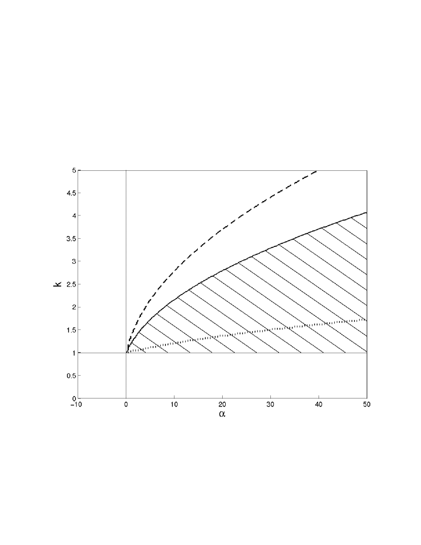
Figure 1: In the shaded region in the plane of the parameters $\left(\alpha\equiv 4k+q,k\right)$, the CW solution (6) of the PI type is stable for $D=1$ [recall that $k$ is the wavenumber of the solution, see Eqs. (2), and $q$ is the phase-mismatch coefficient in Eqs. (1)]. The stability borders of the CW solution for $D=0.5$ and $D=10$ are shown, respectively, by the dashed and dotted curves.

Equation (8) was solved numerically (an analytical solution is formally available, but it takes an intractably complex form). The result, in the form of the stability region of the PI solution, is displayed in Fig. 1. Notice that the solution is always unstable if its wavenumber belongs to the gap of the FF subsystem, which is $k^{2}<1$.

The CW solutions of the PR-type solutions are always modulationally unstable. However, for large values of $|\alpha|$ (actually, in the case of large phase mismatch), the instability band of the perturbation wavenumber $\Omega$ becomes very narrow. For example, it is $8.69<|\Omega|<8.71$ for $\alpha=-100$ and $k=-1.2$. Therefore, the instability generated by a random perturbation will grow very slowly in that case, and, for practical purposes, the CW state may be regarded stable.

The above results pertain to $D=1$ in Eqs. (1). With other values of $D$, we have found that, for the PI-type CWs, the increase of $D$ results in shrinkage of the stability area, and the decrease of $D$ results in its expansion, see the dotted and dashed curves in Fig. 1. The PR-type CW solution remains unstable at any $D$.

4 Dark solitons

4.1 Stationary solitons

The availability of the modulationally-stable CW background suggests a possibility of existence of stable DSs. As concerns search for stationary symmetric ($c=0$) solutions, it is obvious that Eqs. (4) are invariant with respect to the transformation $U\rightarrow U/\sqrt{D}$, $V\rightarrow V$, $\alpha\rightarrow\alpha/D$, and $D\rightarrow 1$, which makes it possible to set $D=1$, varying only $\alpha$ in the stationary equations. Further, we substitute $U(x)=p(x)+ig(x)$, which yields equations for the real functions $p,g$ and $V$,

$$\begin{array}[]{l}p^{\prime}=g(k-1+V),\\ g^{\prime}=-p(k+1+V),\\ V^{\prime\prime}=p^{2}+g^{2}+\alpha V.\end{array}$$ (11)

The SH component can be sought for as $V=V_{0}+\widetilde{V}$, where $V_{0}$ is the CW solution (6) of the PI-type. Then, for the solutions supported by the PI-type CW background, we obtain, from Eqs. (11),

$$p^{\prime} = g\widetilde{V},~{}g^{\prime}=-p(2+\widetilde{V}),$$ (12)

$$\widetilde{V}~{}^{\prime\prime} = p^{2}+g^{2}+\alpha(1-k)+\alpha\widetilde{V}.$$ (13)

Assuming, for the time being, $\left|\widetilde{V}\right|\ll 1$, we approximate the second equation in (12) by $g^{\prime}=-2p$ (the validity of this assumption will be considered later). Then, we look for a fundamental DS solution in the form

$$\begin{array}[]{l}g=\left|U_{0}\right|\tanh(\beta x),~{}p=p_{0}\mathrm{sech}^{2}(\beta x),\\ V=V_{0}+\widetilde{V}_{0}\mathrm{sech}(\beta x),\end{array}$$ (14)

where $U_{0}$ and $V_{0}$ are the same as in Eqs. (6) (hence the solution is matched to the CW background at $x\rightarrow\pm\infty$), while the constants $p_{0},\widetilde{V}_{0}$ and $\beta$ are to be found. Note that, according to Fig. 1, $V_{0}\equiv 1-k$ is negative in the region of stability of the CW background, hence the expression (14) with $\widetilde{V}_{0}>0$ assumes that $\left|V(x)\right|$ has a minimum at $x=0$. Substitution of the ansatz (14) into Eqs. (12) and (13) shows that it solves the first two equations, but not the last one. To identify an approximate solution, we then demand the latter equations to be satisfied only at the central point, $x=0$. This approach leads to a system of algebraic equations, which can be readily solved to yield the following results:

$$\widetilde{V}_{0}=\frac{1}{4}\alpha\left(1-V_{0}/4\right)\left(\sqrt{1-\frac{8V_{0}}{\alpha(1-V_{0}/4)^{2}}}-1\right),$$ (15)

$$\beta=\sqrt{\tilde{V}_{0}},~{}p_{0}=-\frac{1}{2}|U_{0}|\sqrt{\tilde{V}_{0}}$$ (16)

provided that $\tilde{V}_{0}\geq 0$ and $1-\left(8V_{0}/\alpha\right)(1-V_{0}/4)^{-2}\geq 0$. It is straightforward to check that the latter conditions are satisfied in the region of interest ($\alpha>0,k>1$), where the CW solutions of the PI-type are modulationally stable, see Fig. 1.

The above approximation assumed $\widetilde{V}_{0}\ll 1$. To examine the validity of this assumption, we note that the expression (15), considered as a function of $\alpha$, attains the maximum value $\left(\widetilde{V}_{0}\right)_{\max}=4V_{0}/\left(V_{0}-4\right)\equiv 4(k-1)/(3+k)$ at $\alpha=\infty$, hence the assumption is formally justified for small $(k-1)$ (near the upper edge of the spectral gap) if $\alpha$ (i.e., the phase mismatch) is large, and for larger $(k-1)$ if $\alpha$ is smaller.

According to Eqs. (14), the parameters $p_{0}$ and $\widetilde{V}_{0}$ determine the inverse DS contrasts $\sigma_{u,v}$, which may be defined as ratios of the amplitudes at the soliton’s center to those in the CW background: $\sigma_{u}=|p_{0}/U_{0}|$ and $\sigma_{v}=|\widetilde{V}_{0}/V_{0}|$ for the FF and SH, respectively. These parameters belong to the interval $0\leq\sigma_{u,v}\leq 1$, the limiting cases of $\sigma_{u,v}=0$ and $\sigma_{u,v}=1$ corresponding, respectively, to the black soliton, and to the unmodulated CW solution. In particular, Eqs. (15) and (16) predict the black soliton at $\alpha=0$.

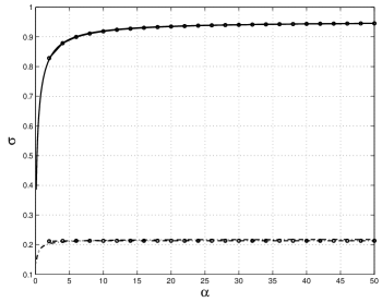
(a) $k=1.2$

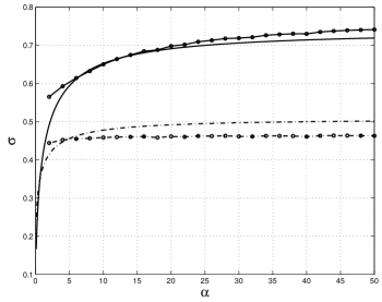
(b) $k=2.4$

Figure 2: The inverse contrasts $\sigma_{u}$ and $\sigma_{v}$ of the fundamental dark soliton supported by the modulationally stable CW background of the PI-type. The solid and dashed-dotted lines show, respectively, the analytical prediction for $\sigma_{v}$ and $\sigma_{u}$; curves of the same types connecting circles show numerical results for $\sigma_{v}$ and $\sigma_{u}$. The panels (a) and (b) pertain to $k=1.2$ and $k=2.4$, and in both cases $D=1$.

The dependences of the inverse contrast on $\alpha$, as obtained from the above approximation and from a direct numerical solution, are shown in Fig. 2 (two cases shown in this figure adequately represent the general situation). The results demonstrate that the analytical approximation is, generally, quite accurate, although numerically found solitons are never completely black. With the increase of $k$, the FF component becomes “grayer”, while the SH one gets darker.

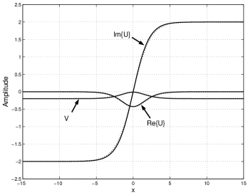
(a) $k=1.2$, $\alpha=20$

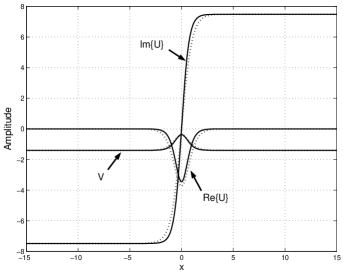
(b) $k=2.4$, $\alpha=40$

Figure 3: Typical examples of the fundamental dark soliton. The solid and dotted lines show, respectively, the numerical solution and the analytical approximation: (a) $k=1.2,\alpha=20$; (b) $k=2.4,\alpha=40$.

Typical examples of the direct comparison between the DS shape, as predicted by the analytical approximation, and as generated by the numerical solution, are displayed in Fig. 3. For $k=1.2$ and $\alpha=20$, the approximation is so close to the exact solution that they are indistinguishable. For $k=2.4$ and $\alpha=40$, the accuracy deteriorates, but the agreement is still fairly good.

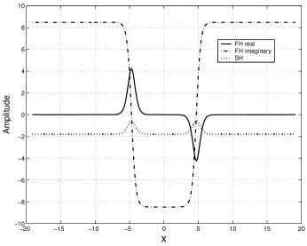
Figure 4: A bound state of two dark solitons, found numerically at $k=2.8$ and $\alpha=40$. In this figure and below, the labels FH and SH pertain, respectively, to the fundamental and second harmonics.

Further numerical search for DS solutions supported by the modulationally stable CW background has revealed the existence of bound states of the DSs, whose shape is similar to that of unstable bound states which were reported Refs. [7] and [14] (however, the bound states may be stable in the present model, see below). Typical examples of twin-hole and tri-hole DS complexes are shown in Figs. 4 and 5.

4.2 Tilted solitons

The general ansatz (2) for steady-shape solutions admits tilted DSs with $c\neq 0$. We have found such solitons by numerical search in the $(k,\alpha)$ plane. The above-mentioned scaling, which allowed us to impose the normalization $D\equiv 1$ for the $c=0$ solitons, does not hold for the tilted ones. Nevertheless, we set $D=1$ in this case too, as the additional problem of scanning the parameter space augmented by the effective diffraction coefficient $D$ is too complex.

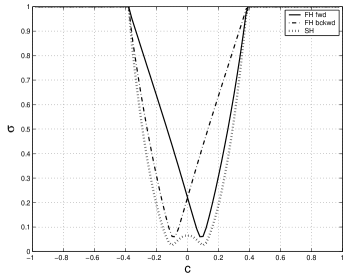
Figure 6: The inverse contrast of three components in the tilted (“moving”) fundamental dark soliton vs. its tilt $c$ for $k=1.2$ and $\alpha=20$. At points $c\equiv c_{\mathrm{bif}}$, where all the three contrasts becomes equal to $1$, the dark soliton disappears, merging into the CW background.

For the tilted DSs, the amplitudes of the two FF components $u_{1}$ and $u_{2}$ are no longer equal, and the SH field $u_{3}$ is not real; accordingly, one should use Eqs. (3) instead of Eqs. (4). Numerical solution for the tilted (“moving”) solitons gives rise to the dependence of the inverse contrasts in the three components (“forward” and “backward” FF ones, and the SH component), defined as above, on the slope (tilt) $c$. A typical result is shown in Fig. 6. For the forward (backward) slope of the DS, the contrast of the forward (backward) FF component initially increases and attains a maximum at some tilt $c_{\max}$. For $\left|c\right|>\left|c_{\max}\right|$, the contrasts of both FF components decrease until the DS reaches a point $c=c_{\mathrm{bif}}$ where $\sigma$ becomes equal to $1$, i.e., the DS disappears, bifurcating back into the CW solution. For the forward-tilted soliton, the forward FF component  of the soliton is always darker than its backward counterpart.

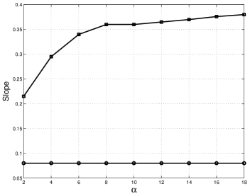
Figure 7: The slope $c_{\mathrm{\min}}$ of the tilted dark soliton, at which the maximum contrast of the soliton’s FF component is achieved (circles), and the slope $c_{\mathrm{bif}}$, at which the dark soliton merges into the CW background (squares), versus the effective mismatch $\alpha$, for $k=1.2$.

The dependence of parameters of the tilted DS on $\alpha$, i.e., on the phase mismatch, is shown in Fig. 7. As is seen, the slope $c_{\max}$, at which the maximum contrast of FF occurs, is virtually independent of $\alpha$. However, the slope $c_{\mathrm{bif}}$ at which the tilted DS bifurcates back into the CW, i.e., the maximum slope past which the DS does not exist, increases with $\alpha$.

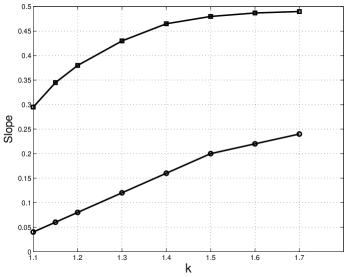
Figure 8: The same as in Fig. 7, but as a function of $k$, for fixed $\alpha=20$.

The dependence of the same parameters on $k$, i.e., as a matter of fact, on the detuning from the gap, is displayed in Fig. 8. As well as it was with the $\alpha$-dependence, the largest FF contrast is independent of $k$, but the corresponding $c_{\max}$ grows with $k$. The bifurcation value $c_{\mathrm{bif}}$ of the tilt is also a growing function of $k$. It was observed too that the maximum values of the contrast remain themselves constant with the variation of both $\alpha$ and $k$.

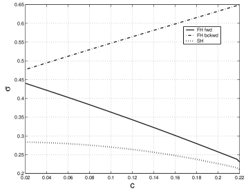
Figure 9: The same as in Fig. 6, but for $k=2.2$.

As $k$ becomes still larger than in the cases like that shown in Fig. 8, viz., at $k>2.1$, the behavior of the DS solution changes drastically. In this region, the numerical scheme ceases to converge close to the bifurcation point, therefore the bifurcation (merger of the DS back into the CW) cannot be identified. A typical example of the dependence of the DS contrast on the tilt for this situation is shown in Fig. 9 (cf. Fig. 6). In this case, the numerical method does not converge for $c>0.22$.

The normalized slope $c$ relates to its physical counterpart $c_{\mathrm{phys}}$, which is the ratio of the real coordinates, as $c_{\mathrm{phys}}=\rho c$, where $\rho$ is the angle between the FF wave vector and the axis $z$. Since the $\rho$ should be small for Eqs. (1) to remain valid, the physical slopes expected to be observed in the experiment are on the order of $10^{-3}-10^{-2}$.

5 Stability and collisions of dark solitons

The stability of the CW background is only a necessary, but not sufficient condition for the stability of DSs. We investigated their full stability by direct simulations, and also through a numerical solution of the eigenvalue problem for small perturbations. In the latter case, the perturbed solution was taken as

$$\begin{array}[]{ccc}u_{1}(x,z)&=&\left[u_{1}^{(0)}(x;k)+\epsilon_{1}(x)\exp(i\lambda z)\right]\exp(ikz),\\ u_{2}(x,z)&=&\left[u_{2}^{(0)}(x;k)+\epsilon_{2}(x)\exp(i\lambda z)\right]\exp(ikz),\\ u_{3}(x,z)&=&\left[u_{3}^{(0)}(x;k)+\epsilon_{3}(x)\exp(i\lambda z)\right]\exp(2ikz),\end{array}$$ (17)

where $u_{n}^{(0)}(x;k)\$represent an unperturbed DS solution, $\epsilon_{n}$ are eigenmodes of infinitesimal perturbations, and $\lambda$ is the corresponding eigenvalue, the stability requiring all $\lambda$ to be real. The expressions (17) were substituted into Eqs. (1), and the resulting equations were linearized in $\epsilon_{n}$.

The problem significantly simplifies for the symmetric solitons with $c=0$, when $u_{1}^{(0)}=-\left(u_{2}^{(0)}\right)^{\ast}$, and $u_{3}^{(0)}$ is real. In that case, we were able to find the full spectrum of the eigenvalues for both the fundamental DSs and their twin-hole bound states (see Fig. 4), on a sufficiently dense grid of points in ($\alpha$,$k$) plane. As in the previous sections, the analysis was restricted to the case of $D=1$, as scanning through the full three-dimensional parametric space including $D$ is a very complex technical problem. As a result, it has been concluded that both the fundamental and twin-hole DSs are always stable, provided that their CW background of the PI type is modulationally stable.

The stability of the symmetric DSs was also verified in direct simulations of Eqs. (1). The verification has shown that they are stable indeed, as predicted by the calculation of the perturbation eigenvalues.

Computation of the stability eigenvalues for the tilted fundamental DSs is too hard to run it in a systematic form. However, their stability can be easily tested in direct simulations. The simulations reveal that, as well as their symmetric (untilted) counterparts, the tilted solitons are  always stable if the CW background is stable.

The stability of the DSs with $c\neq 0$ suggests a possibility to consider “collisions” between them (in fact, intersection between two spatial solitons tilted in opposite directions). The collisions were simulated too, with a conclusion that they always look completely elastic: the DSs re-emerge unaffected after the collision, apart from a displacement of their centers, see an example in Fig. 10. The character of the interaction remains the same for all values of $\alpha$ and $k$ (at least, for the slopes $|c|~{}\geq 0.1$). The collision-induced shift of the centers is (quite naturally) slightly larger for smaller slopes. A typical X-junction formed by the intersection of two dark solitons is shown in Fig. 11.

The collisions are, actually, quite similar to those observed in the integrable NLS model describing dark solitons in a defocusing Kerr medium. As the solitons collide, they repel each other, which is obvious from the contour-plot rendition in Fig. 11. It is relevant to note that interactions between DSs in the integrable self-defocusing NLS equation are repulsive too (see, e.g., Ref. [18]).

We also simulated a different type of interactions between the DS, when two solitons with $c=0$ are originally placed at some distance; obviously, this situation may be relevant to the experiment, and to possible applications. It has been observed that the solitons repel each other in this case as well. With very small radiation loss, they start to “move” (i.e., acquire a finite slope), as is shown in Fig. 12. The eventual slope observed in this set of the simulations virtually does not depend on $k$, and slightly increases with $\alpha$.

6 Conclusions

In this work, we have considered uniform CW states and dark soliton (DSs) in the system of three waves in a planar waveguide [with two fundamental-frequency (FF) and one second-harmonic (SH) components] coupled by the $\chi^{(2)}$ interaction. The FF waves are also linearly coupled by reflections on the Bragg grating. This model was earlier shown to generate a great variety of bright solitons.

We have demonstrated that, on the contrary to the usual situation in spatial-domain $\chi^{(2)}$ models, in the present case CW states with the phase shift $\pi/2$ between the FF and SH waves are modulationally stable in a broad parameter region, provided that the CW wavenumber lies outside the system’s spectral gap. Stationary fundamental DSs supported by the stable CWs were found numerically, and also by means of an ad hoc analytical approximation, which produced results that agree well with numerical findings. Bound states of two and three DSs were found too. The fundamental DSs, as well as dark bi-solitons, are stable in all the cases when the CW background is stable; this was demonstrated by means of calculation of the corresponding stability eigenvalues, and verified in direct simulations.

We have also studied tilted fundamental DSs. It was found that they attain a maximum contrast at a finite value of the slope, that virtually does not depend on the $\chi^{(2)}$ phase mismatch; at a maximum value of the slope (which grows with the mismatch), the DS merges into a CW state. Interactions between tilted solitons were systematically simulated too, with a conclusion that the interactions are repulsive and completely elastic.

References

Figure 5: A typical example of a bound state of three dark solitons, found for $k=2.4$ and $\alpha=20$.

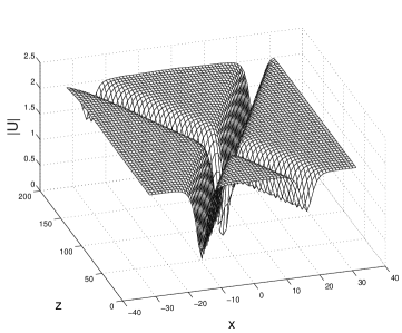
Figure 10: A typical example of the collision between two dark solitons. The slopes are $c=\pm 0.2$, while $k=1.2$ and $\alpha=20$.

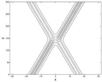
Figure 11: Contour plot of two dark solitons collision showing the displacement of their centers. The slopes are $c=\pm 0.1$, while $k=1.2$ and $\alpha=40$.

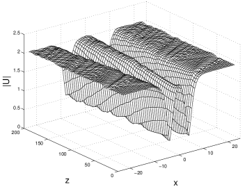
Figure 12: A typical example of the interaction between two dark solitons with the $c=0$ placed initially at some distance from each other. In this case, $k=1.2$ and $\alpha=20$.

References

- [1] Etrich C, Lederer F, Malomed B A, Peschel T and Peschel U 2000 Progr. Opt. 41 483
- [2] Buryak A V, Di Trapani P, Skryabin D V and Trillo S 2002 Phys. Rep. 370 63
- [3] Di Trapani P, Caironi D, Valiulis G, Dubietis A, Danielius R and Piskarskas A 1998 Phys. Rev. Lett. 81 570; Valiulis G, Dubietis A, Danielius R, Caironi D, Visconti A and Di Trapani P 1999 J. Opt. Soc. Am. B 16 722
- [4] Werner M J and Drummond P D 1994 Opt. Lett. 19 613
- [5] Hayata K and Koshiba M 1994 Phys. Rev. A 50 675
- [6] Buryak A V and Kivshar Yu S 1995 Opt. Lett. 20, 834
- [7] Buryak A V and Kivshar Yu S 1995 Phys. Rev. A 51 R41
- [8] Trillo S and Ferro P 1995 Opt. Lett. 20 438
- [9] Kennedy T A B and Trillo S 1996 Phys. Rev. A 54 4396
- [10] He H, Drummond P D and Malomed B A 1996 Opt. Commun. 123 394
- [11] Towers I N, Malomed B A, and Wise F W 2003 Phys. Rev. Lett. 90 123902; Beckwitt K, Chen Y-F, Wise F W, and Malomed B A 2003 Phys. Rev. E 68 057601
- [12] Di Trapani P, Chinaglia W, Minardi S, Piskarskas A, and Valiulis G 2000 Phys. Rev. Lett. 84 3843
- [13] He H, Arraf A, de Sterke C M, Drummond P D and Malomed B A 1999 Phys. Rev. E 59 6064
- [14] Conti C, Trillo S and Assanto G 1997 Phys. Rev. Lett. 78 2341
- [15] Mak W C K, Malomed B A and Chu P L 1998 Phys. Rev. E 58 6708
- [16] Champneys A R and Malomed B A 2000 Phys. Rev. E 61 886
- [17] Schiek R, Baek Y and Stegeman G I 1996 Phys. Rev. E 53 1138; Schiek R, Baek Y, Stegeman G I and Sohler W 1998 Opt. Quant. Electr. 30 861
- [18] Thurston R N and Weiner A M 1991 J. Opt. Soc. Am. B 8 471.