Stability of low-dimensional bushes of vibrational modes in the Fermi-Pasta-Ulam chains

Abstract

Bushes of normal modes represent the exact excitations in the nonlinear physical systems with discrete symmetries [Physica D 117 (1998) 43]. The present paper is the continuation of our previous paper [Physica D 166 (2002) 208], where these dynamical objects of new type were discussed for the monoatomic nonlinear chains. Here, we develop a simple crystallographic method for finding bushes in nonlinear chains and investigate stability of one-dimensional and two-dimensional vibrational bushes for both FPU-$\alpha$ and FPU-$\beta$ models, in particular, of those revealed recently in [Physica D 175 (2003) 31].

1 Introduction

This paper expands upon our previous work [1] where an outline of the general theory of the bushes of modes [2, 3, 4] was presented in connection with the FPU-chain dynamics. Nevertheless, it seems reasonable to recapitulate here some basic notions and ideas.

1.1 The concept of bushes of modes

Bushes of modes can be considered as a new type of exact excitations in nonlinear systems with discrete symmetries, such as molecules and crystals. The simplest way for introducing this concept can be described as follows.

Let us have an $N$-particle Hamiltonian system characterized by a symmetry group $G_{0}$ in its equilibrium state. Let us also assume that this system permits the harmonic approximation and, therefore, we can introduce a complete set of normal modes. Note that every normal mode possesses its own symmetry group $G_{j}$ which is a subgroup of the group $G_{0}$. Let us now excite only one normal mode at the initial instant by imposing the appropriate initial conditions. We call this mode by the term “root mode”. Normal modes are independent of each other in the harmonic approximation. However, if we take into account some anharmonic terms of the Hamiltonian, the excitation will transfer from the root mode to a number of other normal modes with zero amplitudes at the initial instant, so-called “secondary modes”. Because of certain selection rules for the excitation transfer between modes of different symmetry, the number of the secondary modes can often be rather small.

Definition. The complete collection of the root mode and all secondary modes, corresponding to it, forms a bush of normal modes. The number of modes in this collection is the dimension of the given bush.

To avoid any misunderstanding at this point, let us note that one can consider normal modes, determined for a linear system, as a basis for a decomposition of different dynamical regimes in the nonlinear system (for more details, see below).

The energy of the initial excitation turns out to be trapped in the bush simply because of the above definition. The number of modes in the bush does not change in time while the amplitudes of these modes do change.

For many systems, we can find one-dimensional, two-dimensional, three-dimensional and so on bushes of modes. Note that one-dimensional bushes can be treated as the similar nonlinear normal modes introduced by Rosenberg forty years ago [5].

Every bush possesses its own symmetry group $G$ which is a subgroup of the symmetry group of the Hamiltonian of the considered system. In the above discussed case, when the bush is excited by perturbing the root mode, the symmetry group $G$ of the bush coincides with that of this root mode. The symmetries of all other modes of the bush are greater than or equal to its full symmetry $G$. The development of the above ideas leads to the following important statement of the general theory [1, 2, 4]:

Proposition. Different nonlinear dynamical regimes of a physical system can be classified by subgroups of its symmetry group $G_{0}$ (so-called “parent” group).

It is important to emphasize that the considered bushes of modes are symmetry determined objects: the sets of their modes do not depend on the interparticle interactions in the physical system. Taking into account the specific character of these interactions can only reduce the dimension of the bush.

1.2 Some properties of bushes of modes

In general case, we must speak about bushes of symmetry-adapted modes rather than normal modes. Indeed, we consider the symmetry determined bushes whose finding does not need any information about the interactions in the system. The symmetry-adapted coordinates are the basis vectors of the irreducible representations (irreps) of the parent symmetry group $G_{0}$ and they can be found by group-theoretical methods only, without any information about the interactions. In contrast, the normal coordinates, used for construction of normal modes, must be obtained, generally, by diagonalization of the Hamiltonian matrix and, therefore, the interparticle interactions must be taken into account.

In the geometrical sense, a bush of modes is an invariant manifold singled out by its symmetry and decomposed into the basis vectors of the irreducible representations of the appropriate parent symmetry group.

This decomposition plays a very important role in our approach. Indeed, different irreps describe the transformation properties of the dynamical variables corresponding to different physical characteristics of the considered system. For example, some irreps are active in the infrared or Raman experiments, while others are nonactive in optics, but play the essential role in neutronographics, etc.

In this paper, we discuss bushes of vibrational modes describing the time-dependent displacements of the particles of nonlinear chains from their equilibrium positions. Speaking about the symmetry group of a single mode or of the bush as integral object, we mean the specific symmetry of the patterns of the instantaneous displacements of all particles which correspond to the mode or to the bush. Considering the symmetry group of the displacement pattern and the collection of the normal modes contained in a given bush, we deal with the geometrical aspect of the bush. This aspect is independent of the interparticle interactions in the chain.

On the other hand, we deal with the dynamical aspect of the bush when consider the differential equations describing the time-dependence of the amplitudes of the bush modes. In this sense, the given bush represents a reduced dynamical system whose dimension is, in general, less (often, considerably less!) than the dimension of the original physical system. Obviously, the dynamical aspect of the bush, in contrast to the geometrical aspect, depends essentially on the interparticle interactions.

The modes of the bush are coupled by the so-called “force interactions”, while their coupling to all other modes is brought about by “parametric interactions” [4]. The latter interactions can lead to a loss of stability of the bush, if the amplitudes of its modes become sufficiently large [4, 1, 6], because of the phenomenon similar to the well-known parametric resonance. In this case, the spontaneous breaking of the symmetry of the system’s vibrational state takes place and, as a consequence, the given bush transforms into a bush of larger dimension. Precisely this mechanism of stability loss by the bushes of the FPU chains is discussed in this paper. The other mechanisms of the loss of bush stability will be considered elsewhere.

1.3 Some history

The general concept of bushes of modes for physical systems with discrete symmetry was introduced in [2]. Actually, this concept appeared as a generalization of the notion of the complete condensate of primary and secondary order parameters, whose theory was developed in our papers devoted to phase transitions in crystals [7, 8]. The discussion of properties of bushes of modes, the group-theoretical methods for their construction, some theorems about the bush structure can be found in [2, 3, 4]. The bushes of modes for different classes of mechanical systems with point and space symmetry were investigated in [3, 4, 6, 9, 10, 11]. In particular, let us mention the investigation of

– all possible “irreducible bushes” and symmetry determined similar nonlinear normal modes for the mechanical systems with any of the 230 space groups [9];

– low-dimensional bushes for all point groups of crystallographic symmetry [10];

– bushes of vibrational modes for the fullerene $C_{60}$ (“buckyball” structure) [11];

– bushes of modes and their stability for the octahedral structure with Lennard-Jones potential [6].

A review of the group-theoretical methods and the appropriate computer algorithms for treating the condensates of order parameters and bushes of modes can be found in [12]. A remarkable computer program ISOTROPY by Stokes and Hatch, capable to deal with many group-theoretical methods of crystal physics and, in particular, with bushes of modes, is now available on the Internet as free software [13].

In [14], Poggi and Ruffo revealed some exact solutions for the FPU-$\beta$ chain dynamics, by analyzing the appropriate dynamical equations, and investigated their stability. These solutions correspond to certain subsets of normal modes (so-called “subsets of I type”) “where energy remains trapped for suitable initial conditions”.

In [1], we showed that these subsets are the simplest cases of the bushes of modes for the monoatomic nonlinear chains and that they can be found without taking into account the information about the specific interactions in the FPU-$\beta$ model. We discussed there the symmetry-determined bushes of modes with respect to the translational group $T$, in detail, and the bushes with respect to the dihedral group $D$, partially. Also, in the paper [1], the stability of the former bushes for the FPU-$\alpha$ chain was studied.

In a recent paper [15], Bob Rink developed a method for finding all possible symmetric invariant manifolds for the monoatomic chains. In spite of the fact that this paper was carried out independently of our approach, based on the concept of bushes of modes, and that it is written in a more rigorous mathematical style, the main idea and the group-theoretical method are very similar to those in our previous papers. Actually, Bob Rink found all symmetry-determined bushes of modes for the monoatomic chains with respect to the dihedral symmetry group. Moreover, he revealed some bushes for the FPU-$\beta$ chain which are brought about by the additional symmetry of this mechanical system connected with the evenness of its potential (hereafter we call them “additional bushes”). However, let us note that the general idea of the classification of the symmetric manifolds (bushes of modes) by the subgroups of the symmetry group of the Hamiltonian was not emphasized explicitly in this paper.

Finally, we would like to comment on two papers by Shinohara [16], devoted to finding “type I subsets of modes” (bushes, in our terminology) in nonlinear chains with fixed endpoints. The author does not use any symmetry-related method and prefers to analyze the specific structure of the dynamical equations (practically, in the manner similar to that of Poggi and Ruffo in [14]). Moreover, he writes that the “approach, which relies on the direct analysis of the mode-coupling coefficients, is much simpler” than the one based on the group-theoretical methods. In contrast to this opinion, we think that the situation is quite the opposite! In particular, we have tried to demonstrate in the present paper that the symmetry-related methods are much simpler and much more transparent than those based on investigating the structure of the dynamical equations. This simplicity becomes especially apparent when one deals with physical objects more complex than monoatomic chains, such as molecules and crystals characterized by nontrivial symmetry groups.

Note that comparing our results and those from [16], one must take into account that we use periodic boundary conditions, while Shinohara discusses the nonlinear chains with fixed endpoints (the former boundary conditions are more general, since the latter conditions can be considered as their special case). We would also like to note that the stability problem for the bushes of modes (invariant manifolds or “modes subsets of I type”) is not considered in [16]. On the other hand, this problem seems to be important for treating the induction phenomenon discussed in those papers.

1.4 The structure of the present paper

In Section 2, we consider a simple crystallographic method for obtaining bushes of modes in the space of atomic displacements which differ from that in our previous paper [1] and in the paper [15] by Bob Rink. A major advantage of this method is its remarkable clarity. Actually, we obtain the invariant manifolds corresponding to the subgroups of the dihedral group and then decompose them into the normal modes of the monoatomic chain. Here we restrict ourselves to the discussion of one- and two-dimensional bushes only (about other bushes see [17]).

The dynamical description of the bushes of normal modes is presented briefly in Section 3.

The general approach to analyzing the parametric stability of the bushes of normal modes is discussed in Section 4.

Sec. 5 is devoted to investigation of the stability of the one-dimensional (1D) bushes in the FPU-$\alpha$ and FPU-$\beta$ chains. Only one 1D bush, B$[\hat{a}^{2},\hat{i}]$, can be obtained for the monoatomic chain with an even number of particles, if the translational group $T$ is considered as the appropriate parent group of this mechanical system. The stability of the bush B$[\hat{a}^{2},\hat{i}]$ was studied for the FPU-$\alpha$ and FPU-$\beta$ chains in the papers [1] and [14], respectively. However, we obtain some additional one-dimensional bushes considering the dihedral group $D$ as the parent symmetry group [1, 17]. Moreover, as was already mentioned, there exist still more 1D bushes for the FPU-$\beta$ model because of the evenness of its potential [15]. Therefore, it is interesting to compare the regions of stability of all these bushes in both FPU-$\alpha$ and FPU-$\beta$ models. We perform such a comparison in this section. An exceptional case is represented by the bush B$[\hat{a}^{4},\hat{a}\hat{i}]$ for the FPU-$\alpha$ chain for which the threshold of stability loss is exactly equal to zero (this result can be proved analytically).

We discuss here the stability of 1D bushes not only for the FPU chains with the finite number of particles ($N$), but for the continuum limit ($N\rightarrow\infty$), as well.

In Section 6 we discuss the shape of the stability regions of the two-dimensional (2D) bushes for the FPU-$\alpha$ and FPU-$\beta$ chains. Indeed, thresholds of the loss of stability of the 1D bushes depend only on their energy, while the similar thresholds for multi-dimensional bushes depend on the complete set of the initial conditions for the dynamical equations of the bush. We demonstrate, with the aid of the appropriate plots, how nontrivial the stability regions of the 2D bushes for the FPU chains can be. The dependence of these regions on the total number of particles in the chains is partially discussed.

In Conclusion (Sec. 7), the obtained results are summarized and some new directions for the bush theory are outlined.

2 Simple crystallographic method for finding bushes of vibrational modes in the monoatomic chains

We consider the longitudinal vibrations of $N$-particle monoatomic chains with periodic boundary conditions. Let the $N$-dimensional vector

$$\bm{X}(t)=\{x_{1}(t),x_{2}(t),\dotsc,x_{N}(t)\}$$

describe all the displacements, $x_{i}(t)$, of the individual particles (atoms) from their equilibrium states at the instant $t$. In accordance with the above-mentioned periodic boundary conditions, we demand for arbitrary time $t$:

$$x_{N+1}(t)\equiv x_{1}(t).$$ (1)

In the equilibrium state, a given chain is invariant under the action of the operator $\hat{a}$ which shifts the chain by the lattice spacing $a$. This operator generates the translational group

$$T=\{\hat{E},\hat{a},\hat{a}^{2},\dotsc,\hat{a}^{N-1}\},\quad\hat{a}^{N}=\hat{E},$$ (2)

where $\hat{E}$ is the identity element and $N$ is the order of the cyclic group $T$. The operator $\hat{a}$ induces the cyclic permutation of all particles of the chain and, therefore, it acts on the “configuration vector” $\bm{X}(t)$ as follows:

$$\hat{a}\bm{X}(t)\equiv\hat{a}\{x_{1}(t),x_{2}(t),\dotsc,x_{N-1}(t),x_{N}(t)\}=\{x_{N}(t),x_{1}(t),x_{2}(t),\dotsc,x_{N-1}(t)\}.$$

The full symmetry group of the monoatomic chain contains also the inversion $\hat{i}$, with respect to the center of the chain, which acts on the vector $\bm{X}(t)$ in the following manner:

$$\hat{i}\bm{X}(t)\equiv\hat{i}\{x_{1}(t),x_{2}(t),\dotsc,x_{N-1}(t),x_{N}(t)\}=\{-x_{N}(t),-x_{N-1}(t),\dotsc,-x_{2}(t),-x_{1}(t)\}.$$

The complete set of all products $\hat{a}^{k}\hat{i}$ of the pure translations $\hat{a}^{k}$ ($k=1,2,\dotsc,N-1$) with the inversion $\hat{i}$ forms the so-called dihedral group $D$ which can be written as a direct sum of two cosets $T$ and $T\cdot\hat{i}$:

$$D=T\oplus T\cdot\hat{i}.$$ (3)

The dihedral group is non-Abelian group induced by two generators ($\hat{a}$ and $\hat{i}$) with the following generating relations

$$\hat{a}^{N}=\hat{E},\quad\hat{i}^{2}=\hat{E},\quad\hat{i}\hat{a}=\hat{a}^{-1}\hat{i}.$$ (4)

Let us consider the geometrical interpretation of the symmetry elements of the dihedral group $D$. For simplification, we will use the reflection $\hat{\sigma}$ in the mirror plane orthogonal to the chain instead of the inversion $\hat{i}$. Indeed, the actions of $\hat{\sigma}$ and $\hat{i}$ on the vectors of the one-dimensional space are equivalent to each other ($\hat{\sigma}x=\hat{i}x=-x$). Then we can use the well-known theorem of crystallography: “Any mirror plane and the translation $\bm{A}$ orthogonal to it generate a new mirror plane, parallel to the former plane and displaced away from it by $\bm{A}/2$”.

Let the number of particles in the chain ($N$) be an even integer. Then it is easy to check that the products $\hat{a}^{k}\hat{\sigma}\equiv\hat{a}^{k}\hat{i}$ ($k=\pm 1,\pm 2,\pm 3,\dotsc$) generate the family of parallel planes depicted by vertical lines in Fig. 1. For odd $k$, these planes pass through the atoms, while for the even $k$ they pass between atoms, exactly at the middle of the neighboring particles. Note that, for odd $N$, everything will be vice versa: for even $k$, the planes pass through the atoms and for the add $k$ – between them. In Fig. 1, we show a part of the family of the above mentioned planes near the center of the chain. It can be verified that the symmetry elements $\hat{a}^{k}\hat{\sigma}\equiv\hat{a}^{k}\hat{i}$ ($k=1,2,3,\dotsc$) are located to the right of the center of the chain, while the elements $\hat{\sigma}\hat{a}^{k}\equiv\hat{i}\hat{a}^{k}$ are located to the left from it.

Figure 1: Symmetry elements of the dihedral group $D$ near the center of the monoatomic chain.

Let us now consider the subgroups $G_{j}$ of the dihedral group $D$, keeping in mind that every subgroup $G_{j}\subset D$ induces the certain bush of modes.

Each group $G_{j}$ contains its own translational subgroup $T_{j}\subset T$, where $T$ is the above discussed full translational group (2). If $N$ is divisible by 4 (for example, we consider below the case $N=12$) there exists the subgroup $T_{4}=[\hat{a}^{4}]$ of the group $T=[\hat{a}]$. Note that in square brackets we write down only generators of the considered group, while the complete set of group elements is written in curly brackets (see, for example, Eqs. (2)).

If a vibrational state of the chain possesses the symmetry group $T_{4}=[\hat{a}^{4}]\equiv\{\hat{E},\hat{a}^{4},\hat{a}^{8},\dotsc,\hat{a}^{N-4}\}$, displacements of the atoms, which are apart by the distance $4a$ from each other in the equilibrium state, turn out to be equal. Therefore, for the case $N=12$, we can write the following atomic displacement pattern:

$$\bm{X}(t)=\{x_{1}(t),x_{2}(t),x_{3}(t),x_{4}(t)~{}|~{}x_{1}(t),x_{2}(t),x_{3}(t),x_{4}(t)~{}|~{}x_{1}(t),x_{2}(t),x_{3}(t),x_{4}(t)\},$$ (5)

where $x_{i}(t)$ ($i=1,2,3,4$) are arbitrary functions of time. The pattern (5) determines the bush corresponding to the symmetry group $T_{4}=[\hat{a}^{4}]$. Thus, the complete set of the atomic displacements can be divided into $N/4$ (in our case, $N/4=3$) identical subsets, and each of them determines the so-called “Extended Primitive Cell” (EPC). For the bush (5), the EPC contains four atoms, and the vibrational state of the whole chain is described by three such EPC. In other words, the EPC for the vibrational state with the symmetry group $T_{4}=[\hat{a}^{4}]$ (its size is equal to $4a$) is four times larger than the primitive cell ($a$) of the chain in the equilibrium state.

It is essential that some symmetry elements of the dihedral group $D$ disappear as a result of the symmetry reduction $D=[\hat{a},\hat{i}]\rightarrow T_{4}=[\hat{a}^{4}]$. In our case, there are no nontrivial symmetry elements of the group $D$ inside the EPC and, as a consequence, there are no restrictions on the displacements belonging to one and the same extended cell (this fact is obvious from Eq. (5)).

There are four other subgroups of the dihedral group $D$ to which the same translational subgroup $T_{4}=[\hat{a}^{4}]$ correspond:

$$[\hat{a}^{4},\hat{i}],\quad[\hat{a}^{4},\hat{a}\hat{i}],\quad[\hat{a}^{4},\hat{a}^{2}\hat{i}],\quad[\hat{a}^{4},\hat{a}^{3}\hat{i}].$$ (6)

These subgroups possess two generators, namely, the common translational generator $\hat{a}^{4}$ and different inversion elements $\hat{a}^{k}\hat{i}$ ($k=0,1,2,3$). These inversion elements differ from each other by the position of the center of inversion (see Fig. 1 where they are depicted by the vertical lines representing the mirror planes).

Note that subgroups $[\hat{a}^{4},\hat{a}^{k}\hat{i}]$ with $k>3$ are equivalent to those from the list (6), because the second generator $\hat{a}^{k}\hat{i}$ can be multiplied by $\hat{a}^{-4}$, representing the inverse element with respect to the first generator $\hat{a}^{4}$. Thus, there exist only five subgroups of the dihedral group (with $N\mod 4=0$) constructed on the basis of the translational group $T_{4}=[\hat{a}^{4}]$, namely, this group and the four groups from the list (6).

Now, let us consider the bushes corresponding to the subgroups (6).

1. The subgroup $[\hat{a}^{4},\hat{i}]$ consists of the following six elements:

$$\hat{E},\hat{a}^{4},\hat{i},\hat{a}^{4}\hat{i},\hat{a}^{8}\hat{i}\equiv\hat{i}\hat{a}^{4}.$$ (7)

The diagram of this subgroup, similar to that of the full dihedral group $D$ in Fig. 1, is depicted in Fig. 2.

Figure 2: Vibrational bush corresponding to the subgroup $G=[\hat{a}^{4},\hat{i}]$.

Two symmetry elements ($\hat{i}\hat{a}^{4}$ and $\hat{a}^{4}\hat{i}$), situated at the boundaries of the EPC, do not produce any additional restrictions on the atomic displacements inside this EPC. Indeed, they connect with each other the atomic displacements in the adjacent extended primitive cells, while the equivalence of the displacements of the atoms with the same positions in the adjacent EPC is guaranteed by the translation $\hat{a}^{4}$ which is the first generator of the considered subgroup $[\hat{a}^{4},\hat{i}]$.

On the other hand, the inversion $\hat{i}$ at the center of the EPC (Fig. 2), surviving in the subgroup $[\hat{a}^{4},\hat{i}]$, demands the displacements of the atoms, symmetrically situated with respect to this center, to be equal in value, but opposite in sign:

$$x_{1}(t)=-x_{4}(t),\quad x_{2}(t)=-x_{3}(t).$$ (8)

These relations between the atomic displacements are shown in Fig. 2 by the appropriate arrows. As a consequence, the atomic displacements, corresponding to the bush B$[\hat{a}^{4},\hat{i}]$ with the symmetry group $[\hat{a}^{4},\hat{i}]$, can be written (for $N=12$) in the following form:

$$\bm{X}(t)=\{x_{1}(t),x_{2}(t),-x_{2}(t),-x_{1}(t)~{}|~{}x_{1}(t),x_{2}(t),-x_{2}(t),-x_{1}(t)~{}|~{}x_{1}(t),x_{2}(t),-x_{2}(t),-x_{1}(t)\}$$ (9)

Since Eqs. (8) hold for an arbitrary moment $t$, we will drop the argument $t$ and write down the vibrational bush in the $X$-space (configuration space) as follows:

$$\text{B}[\hat{a}^{4},\hat{i}]=|x_{1},x_{2},-x_{2},-x_{1}|.$$ (10)

Thus, we point out the atomic displacements in only one EPC.

2. For the subgroup

$$[\hat{a}^{4},\hat{a}\hat{i}]\equiv\{\hat{E},\hat{a}^{4},\hat{a}^{8},\hat{a}\hat{i},\hat{a}^{5}\hat{i}\equiv\hat{i}\hat{a}^{7},\hat{a}^{9}\hat{i}\equiv\hat{i}\hat{a}^{3}\},$$ (11)

we obtain the diagram depicted in Fig. 3. In this diagram, one can see two symmetry elements, $\hat{i}\hat{a}^{3}$ and $\hat{a}\hat{i}$, which pass, respectively, through the first and third atoms of the represented EPC. Therefore, the displacements of these atoms must satisfy the relations $x_{1}(t)=-x_{1}(t)$, $x_{3}(t)=-x_{3}(t)$. In turn, this means that $x_{1}(t)\equiv 0$, $x_{3}(t)\equiv 0$, i.e. the atoms located on the inversion elements (which are equivalent, in the one-dimensional space, to the mirror planes!) must be immovable.

Figure 3: Vibrational bush corresponding to the subgroup $G=[\hat{a}^{4},\hat{a}\hat{i}]$.

On the other hand, the symmetry element $\hat{a}\hat{i}$ is situated in the middle between the second and fourth atoms of the EPC and, therefore, their possible displacements must satisfy the equation $x_{2}(t)=-x_{4}(t)$. Thus, we have the following displacement pattern for the bush B$[\hat{a}^{4},\hat{a}\hat{i}]$

$$\bm{X}(t)=\{0,x(t),0,-x(t)~{}|~{}0,x(t),0,-x(t)~{}|~{}0,x(t),0,-x(t)\}$$ (12)

with only one independent dynamical variable $x(t)$. We can write this one-dimensional vibrational bush in the abbreviated form:

$$\text{B}[\hat{a}^{4},\hat{a}\hat{i}]=|0,x,0,-x|.$$

3. The diagram of the symmetry elements of the subgroup

$$[\hat{a}^{4},\hat{a}^{2}\hat{i}]\equiv\{\hat{E},\hat{a}^{4},\hat{a}^{8},\hat{a}^{2}\hat{i},\hat{a}^{6}\hat{i}\equiv\hat{i}\hat{a}^{6},\hat{a}^{10}\hat{i}\equiv\hat{i}\hat{a}^{2}\}$$

is depicted in Fig. 4.

Figure 4: Vibrational bush corresponding to the subgroup $G=[\hat{a}^{4},\hat{a}^{2}\hat{i}]$.

There are two elements, $\hat{i}\hat{a}^{2}$ and $\hat{a}^{2}\hat{i}$ surviving in the transition from the full dihedral group $D=[\hat{a},\hat{i}]$ to the considered subgroup $[\hat{a}^{4},\hat{a}^{2}\hat{i}]$. These elements are located between two first and two last atoms of the depicted EPC. Therefore, $x_{1}(t)=-x_{2}(t)$, $x_{3}(t)=-x_{4}(t)$ and the corresponding displacement pattern is

$$\bm{X}(t)=\{x_{1}(t),-x_{1}(t),x_{2}(t),-x_{2}(t)~{}|~{}x_{1}(t),-x_{1}(t),x_{2}(t),-x_{2}(t)~{}|~{}x_{1}(t),-x_{1}(t),x_{2}(t),-x_{2}(t)\}.$$ (13)

There are two degrees of freedom in (13), $x_{1}(t)$ and $x_{2}(t)$. Thus, the two-dimensional bush with the symmetry group $[\hat{a}^{4},\hat{a}^{2}\hat{i}]$ can be written as

$$\text{B}[\hat{a}^{4},\hat{a}^{2}\hat{i}]=|x_{1},-x_{1},x_{2},-x_{2}|.$$

4. The diagram of the symmetry elements for the last subgroup of the list (6)

$$[\hat{a}^{4},\hat{a}^{3}\hat{i}]\equiv\{\hat{E},\hat{a}^{4},\hat{a}^{8},\hat{a}^{3}\hat{i},\hat{a}^{7}\hat{i}\equiv\hat{i}\hat{a}^{5},\hat{a}^{11}\hat{i}\equiv\hat{i}\hat{a}\}$$

is depicted in Fig. 5.

Figure 5: Vibrational bush corresponding to the subgroup $G=[\hat{a}^{4},\hat{a}^{3}\hat{i}]$.

We see from this diagram that $x_{2}(t)\equiv 0$, $x_{4}(t)\equiv 0$, $x_{1}(t)=-x_{3}(t)$, and, therefore,

$$\bm{X}(t)=\{x(t),0,-x(t),0~{}|~{}x(t),0,-x(t),0~{}|~{}x(t),0,-x(t),0\}.$$ (14)

The corresponding one-dimensional bush can be written as follows

$$\text{B}[\hat{a}^{4},\hat{a}^{2}\hat{i}]=|x,0,-x,0|.$$

We have just considered all the subgroups of the dihedral group $D$, which contain the common translational group $T_{4}=[\hat{a}^{4}]$, and the corresponding vibrational bushes. In the same way, we can find the subgroups of the group $D$ corresponding to the arbitrary translational group $T_{m}=[\hat{a}^{m}]$ and then obtain the bushes induced by these subgroups [17]. We will not discuss this method any further in the present paper, because all the bushes of modes (symmetric invariant manifolds) for the dihedral group were recently obtained by Bob Rink in [15]. Nevertheless, let us note that the above described crystallographic method for finding bushes of vibrational modes seems to be more straightforward than that used in [15]. Actually, the former method represents a variant of our general method of the splitting of the space group orbits (SO) [12, 8], adapted for the sufficiently simple case of the dihedral group $D$. The SO method was developed for finding the so-called complete condensate of primary and secondary order parameters in the framework of the theory of phase transitions in crystals. It was applied to such nontrivial space groups as $O_{h}^{1}$ [8], $O_{h}^{7}$ [19], etc.

The notion of the complete condensate of order parameters is equivalent to the notion of the bush of modes in the geometrical (only geometrical!) sense. Three different methods for finding the condensate of order parameters were considered in [7, 12, 8]: the “direct method”, which is similar to that by Bob Rink [15], the above mentioned SO method and the method based on the concept of the irreducible representations of the appropriate symmetry groups. The last method was used, in particular, for treating bushes of vibrational modes in nonlinear chains in the paper [1].

Now let us consider the notion of the bush equivalence. There are two pairs of equivalent bushes of modes induced by the subgroups from the list (6). Indeed, shifting the displacement pattern (12) of the bush B$[\hat{a}^{4},\hat{a}\hat{i}]$ by the lattice spacing $a$, we obtain the displacement pattern (14) of the bush B$[\hat{a}^{4},\hat{a}^{3}\hat{i}]$. The pattern (9) of the bush B$[\hat{a}^{4},\hat{i}]$ can be transformed into the pattern (13) of the bush B$[\hat{a}^{4},\hat{a}^{2}\hat{i}]$ by the same shifting.

The importance of the notion of bush equivalence is brought about by the fact that equivalent bushes represent identical dynamical systems: they are described by equivalent equations of motions (see below). It can be proved, in the general case, that the conjugate subgroups of the parent symmetry group induce equivalent bushes. Remember that two subgroups $G_{1}$ and $G_{2}$ of the same group $G$ ($G_{1}\subset G$, $G_{2}\subset G$) are called conjugate to each other ($G_{1}\sim G_{2}$), if there exists at least one element $g_{0}$ of the group $G$ which transfers $G_{1}$ into $G_{2}$ by the transformation

$$G_{2}=g_{0}^{-1}G_{1}g_{0}\quad(g_{0}\in G).$$ (15)

It can be easy checked the following conjugations:

$$\left[\hat{a}^{4},\hat{i}\right]\sim\left[\hat{a}^{4},\hat{a}^{2}\hat{i}\right],\quad\left[\hat{a}^{4},\hat{a}\hat{i}\right]\sim\left[\hat{a}^{4},\hat{a}^{3}\hat{i}\right].$$ (16)

For example, using Eqs. (4), we obtain the relation

$$[\hat{a}^{4},\hat{a}\hat{i}]=\hat{a}^{-1}\cdot[\hat{a}^{4},\hat{a}^{3}\hat{i}]\cdot a,$$

which proves the equivalence of the subgroups $[\hat{a}^{4},\hat{a}\hat{i}]$ and $[\hat{a}^{4},\hat{a}^{3}\hat{i}]$, if we take into account the definition (15) with $g_{0}=\hat{a}$. Thus, the both above considered one-dimensional bushes B$[\hat{a}^{4},\hat{a}\hat{i}]$ and B$[\hat{a}^{4},\hat{a}^{3}\hat{i}]$ turn out to be equivalent to each other, as well as the both two-dimensional bushes, B$[\hat{a}^{4},\hat{i}]$ and B$[\hat{a}^{4},\hat{a}^{2}\hat{i}]$. Moreover, it can be proved that for any even $m$ and $k=0,1,2,\dotsc,m-1$, all bushes of the form B$[\hat{a}^{m},\hat{a}^{k}\hat{i}]$ with $k$ of the same evenness are equivalent. For odd $m$, all the bushes of this form are equivalent.

Let us summarize the above said about the construction of the vibrational bushes for nonlinear monoatomic chains.

– Each subgroup of the dihedral group singles out a certain bush of vibrational modes.

– Every subgroup is determined by one or two generators and contains the translational subgroup $T_{k}=[\hat{a}^{k}]$ (it is trivial, $T_{0}$, for the subgroups $[\hat{a}^{m}\hat{i}]$, $m=0,1,2,\dotsc,N-1$).

– The translational subgroup $T_{k}=[\hat{a}^{k}]$ determines the extended primitive cell (EPC) for the vibrational state of the chain.

– The symmetry elements $\hat{a}^{m}\hat{i}$, belonging to the second coset of the dihedral group (see Eq. (3)) and surviving at the symmetry lowering $D\equiv[\hat{a},\hat{i}]\rightarrow[\hat{a}^{k},\hat{a}^{m}\hat{i}]$, produce certain restrictions on the displacements inside the EPC.

– The conjugate subgroups induce the equivalent bushes of modes. The number of the equivalent bushes of a given type is equal to the index of the corresponding subgroup in the dihedral group.

In addition, note that there exist subgroups to which no vibrational bushes correspond. In our case, the subgroup $[\hat{a}^{2},\hat{a}\hat{i}]$ does not induce the vibrational bush, because the EPC, corresponding to this subgroup, contains only two atoms through which the inversion elements, $\hat{i}\hat{a}$ and $\hat{a}\hat{i}$, pass and, therefore, these atoms cannot move.

The bushes obtained with the aid of the described method represent invariant manifolds determined in the configuration space. Let us now consider the bushes in the modal space.

We consider the normal modes for the monoatomic chain in the form used in [14]:

$$\bm{\psi}_{k}=\left\{\frac{1}{\sqrt{N}}\left.\left[\sin\left(\frac{2\pi k}{N}n\right)+\cos\left(\frac{2\pi k}{N}n\right)\right]\right|n=1,2,\dotsc,N\right\}.$$ (17)

Here the subscript $k$ refers to the mode, while the subscript $n$ refers to the atom. The modes $\bm{\psi}_{k}$ ($k=0,1,2,\dotsc,N-1$) form an orthonormal basis in the modal space and we can decompose the set of the atomic displacements $\bm{X}(t)$, corresponding to a given bush, in this basis

$$\bm{X}(t)=\sum_{k=0}^{N-1}\nu_{k}(t)\bm{\psi}_{k}$$ (18)

For example, we obtain the following decompositions for the bushes B$[\hat{a}^{4},\hat{i}]$ and B$[\hat{a}^{4},\hat{a}^{2}\hat{i}]$:

$$\bm{X}(\text{B}[\hat{a}^{4},\hat{i}]) \equiv \{x_{1}(t),x_{2}(t),-x_{1}(t),-x_{2}(t)|x_{1}(t),x_{2}(t),-x_{1}(t),-x_{2}(t)|x_{1}(t),x_{2}(t),-x_{1}(t),-x_{2}(t)\}$$ (19)

$$= \mu(t)\bm{\psi}_{N/2}+\nu(t)\bm{\psi}_{3N/4},$$

$$\bm{X}(\text{B}[\hat{a}^{4},\hat{a}^{2}\hat{i}]) = \tilde{\mu}(t)\bm{\psi}_{N/2}+\tilde{\nu}(t)\bm{\psi}_{N/4}.$$ (20)

Only vectors $\bm{\psi}_{N/2}$, $\bm{\psi}_{N/4}$ and $\bm{\psi}_{3N/4}$ from the complete basis (17) contribute to these two-dimensional bushes:

$$\bm{\psi}_{N/2} = \frac{1}{\sqrt{N}}(-1,1,-1,1,-1,1,-1,1,-1,1,-1,1),$$ (21)

$$\bm{\psi}_{N/4} = \frac{1}{\sqrt{N}}(1,-1,-1,1,1,-1,-1,1,1,-1,-1,1),$$ (22)

$$\bm{\psi}_{3N/4} = \frac{1}{\sqrt{N}}(-1,-1,1,1,-1,-1,1,1,-1,-1,1,1).$$ (23)

Remember that these bushes are equivalent to each other, i.e. they represent the so-called “dynamical domains”. For the bush B$[\hat{a}^{4},\hat{i}]$ we can find the following relations between the old dynamical variables $x_{1}(t)$, $x_{2}(t)$ (relating to the configuration space) and the new dynamical variables $\mu(t)$, $\nu(t)$ (relating to the modal space):

$$\begin{array}[]{l}\mu(t)=-\frac{\sqrt{N}}{2}[x_{1}(t)-x_{2}(t)],\\ \nu(t)=-\frac{\sqrt{N}}{2}[x_{1}(t)+x_{2}(t)].\end{array}$$ (24)

Thus, each of the above bushes consists of two modes. One of these modes is the root mode ($\bm{\psi}_{3N/4}$ for the bush B$[\hat{a}^{4},\hat{i}]$ and $\bm{\psi}_{N/4}$ for the bush B$[\hat{a}^{4},\hat{a}^{2}\hat{i}]$), while the other mode $\bm{\psi}_{N/2}$ is the secondary mode. Indeed, we have already discussed (see Introduction) that the symmetry of the secondary modes must be higher or equal to the symmetry of the root mode. In our case, as it can be seen from Eqs. (22), the translational symmetry of the mode $\bm{\psi}_{N/4}$ is $\hat{a}^{4}$ (acting by this element on (22) we obtain the same displacement pattern), while the translational symmetry of the mode $\bm{\psi}_{N/2}$ is $\hat{a}^{2}$, which is two times higher than that of $\bm{\psi}_{N/4}$ (see (21)-(23)).

One-dimensional (1D) and two-dimensional (2D) vibrational bushes for the FPU chains in configuration and modal spaces can be seen in Tables 1,2. Note that in these tables, as well as in Tables 3,4,5 we list one-dimensional bushes completely, but two-dimensional bushes partially: only those 2D bushes are given whose stability properties are studied in the present paper (see Sec. 6). The complete list of 2D bushes in the FPU chains can be found in Appendix.

Table 1: Representation of 1D and 2D bushes of vibrational modes for the FPU chains in the configuration space (classification by the dihedral group $D$)

Bush	Displacement pattern	Dimension
B$[a^{2},i]$	$|x,-x|$	1
B$[a^{3}]$	$|x_{1},x_{2},x_{3}|^{*}$	2
B$[a^{3},i]$	$|x,0,-x|$	1
B$[a^{3},ai]$	$|0,x,-x|$	1
B$[a^{3},a^{2}i]$	$|x,-x,0|$	1
B$[a^{4},i]$	$|x_{1},x_{2},-x_{2},-x_{1}|$	2
B$[a^{4},a^{2}i]$	$|x_{1},-x_{1},x_{2},-x_{2}|$	2
B$[a^{4},ai]$	$|0,x,0,-x|$	1
B$[a^{4},a^{3}i]$	$|x,0,-x,0|$	1
B$[a^{6},ai]$	$|0,x_{1},x_{2},0,-x_{2},-x_{1}|$	2
B$[a^{6},a^{3}i]$	$|x_{1},0,-x_{1},x_{2},0,-x_{2}|$	2
B$[a^{6},a^{5}i]$	$|x_{1},x_{2},0,-x_{2},-x_{1},0|$	2

^∗ Here $x_{3}$ is not an independent variable: its value must be determined by the condition of immobility of the mass center of the chain, $x_{1}+x_{2}+x_{3}=0$.

Table 2: Representation of 1D and 2D bushes of vibrational modes for the FPU chains in the modal space (classification by the dihedral group $D$). Here $\varepsilon_{1}=\sin\left(\frac{\pi}{12}\right)=\frac{\sqrt{2}(\sqrt{3}-1)}{4}$, $\varepsilon_{2}=\cos\left(\frac{\pi}{12}\right)=\frac{\sqrt{2}(\sqrt{3}+1)}{4}$, $\varepsilon_{3}=\frac{\sqrt{2}}{2}$

Bush	Representation in modal space
B$[a^{2},i]$	$\nu\bm{\psi}_{N/2}$
B$[a^{3},i]$	$\nu(\varepsilon_{1}\bm{\psi}_{N/3}+\varepsilon_{2}\bm{\psi}_{2N/3})$
B$[a^{3},ai]$	$\nu(\varepsilon_{2}\bm{\psi}_{N/3}+\varepsilon_{1}\bm{\psi}_{2N/3})$
B$[a^{3},a^{2}i]$	$\nu\varepsilon_{3}(\bm{\psi}_{N/3}-\bm{\psi}_{2N/3})$
B$[a^{4},i]$	$\nu_{1}\bm{\psi}_{3N/4}-\nu_{2}\bm{\psi}_{N/2}$
B$[a^{4},a^{2}i]$	$\nu_{1}\bm{\psi}_{N/4}+\nu_{2}\bm{\psi}_{N/2}$
B$[a^{4},ai]$	$\nu\varepsilon_{3}(\bm{\psi}_{N/4}+\bm{\psi}_{3N/4})$
B$[a^{4},a^{3}i]$	$\nu\varepsilon_{3}(\bm{\psi}_{N/4}-\bm{\psi}_{3N/4})$
B$[a^{6},ai]$	$\nu_{1}(\varepsilon_{1}\bm{\psi}_{N/6}+\varepsilon_{2}\bm{\psi}_{5N/6})+\nu_{2}(-\varepsilon_{2}\bm{\psi}_{N/3}-\varepsilon_{1}\bm{\psi}_{2N/3})$
B$[a^{6},a^{3}i]$	$\nu_{1}(\varepsilon_{2}\bm{\psi}_{N/6}+\varepsilon_{1}\bm{\psi}_{5N/6})+\nu_{2}(\varepsilon_{1}\bm{\psi}_{N/3}+\varepsilon_{2}\bm{\psi}_{2N/3})$
B$[a^{6},a^{5}i]$	$\nu_{1}\varepsilon_{3}(\bm{\psi}_{N/6}-\bm{\psi}_{5N/6})+\nu_{2}\varepsilon_{3}(\bm{\psi}_{N/3}-\bm{\psi}_{2N/3})$

Table 3: Additional 1D and 2D bushes, for the FPU-$\beta$ chain (these bushes were obtained in [15])

Bush	Dim.	Displacement pattern	Representation in the modal space
B$[a^{3},iu]$ B$[a^{3},aiu]$ B$[a^{3},a^{2}iu]$	1	$|x,-2x,x|$ $|-2x,x,x|$ $|x,x,-2x|$	$\nu(\varepsilon_{2}\bm{\psi}_{N/3}-\varepsilon_{1}\bm{\psi}_{2N/3})$ $\nu(\varepsilon_{1}\bm{\psi}_{N/3}-\varepsilon_{2}\bm{\psi}_{2N/3})$ $\nu\varepsilon_{3}(\bm{\psi}_{N/3}+\bm{\psi}_{2N/3})$
B$[a^{4},iu]$ B$[a^{4},a^{2}iu]$	1	$|x,-x,-x,x|$ $|x,x,-x,-x|$	$\nu\bm{\psi}_{N/4}$ $\nu\bm{\psi}_{3N/4}$
B$[a^{6},ai,a^{3}u]$ B$[a^{6},a^{3}i,a^{3}u]$ B$[a^{6},a^{5}i,a^{3}u]$	1	$|0,x,x,0,-x,-x|$ $|x,0,-x,-x,0,x|$ $|x,x,0,-x,-x,0|$	$\nu(\varepsilon_{1}\bm{\psi}_{N/6}+\varepsilon_{2}\bm{\psi}_{5N/6})$ $\nu(\varepsilon_{2}\bm{\psi}_{N/6}+\varepsilon_{1}\bm{\psi}_{5N/6})$ $\nu\varepsilon_{3}(\bm{\psi}_{N/6}-\bm{\psi}_{5N/6})$
B$[a^{4},aiu]$ B$[a^{4},a^{3}iu]$	2	$|x_{1},x_{2},x_{3},x_{2}|^{**}$ $|x_{2},x_{1},x_{2},x_{3}|^{**}$	$\nu_{1}\varepsilon_{3}(\bm{\psi}_{N/4}-\bm{\psi}_{3N/4})+\nu_{2}\bm{\psi}_{N/2}$ $\nu_{1}\varepsilon_{3}(\bm{\psi}_{N/4}+\bm{\psi}_{3N/4})+\nu_{2}\bm{\psi}_{N/2}$
B$[a^{4},a^{2}u]$	2	$|x_{1},x_{2},-x_{1},-x_{2}|$	$\nu_{1}\bm{\psi}_{N/4}+\nu_{2}\bm{\psi}_{3N/4}$
B$[a^{6},iu]$ B$[a^{6},a^{2}iu]$ B$[a^{6},a^{4}iu]$	2	$|x_{1},x_{2},x_{3},x_{3},x_{2},x_{1}|^{**}$ $|x_{1},x_{1},x_{2},x_{3},x_{3},x_{2}|^{**}$ $|x_{1},x_{2},x_{2},x_{1},x_{3},x_{3}|^{**}$	$\nu_{1}(\varepsilon_{2}\bm{\psi}_{N/6}+\varepsilon_{1}\bm{\psi}_{5N/6})+\nu_{2}(\varepsilon_{2}\bm{\psi}_{N/3}-\varepsilon_{1}\bm{\psi}_{2N/3})$ $\nu_{1}\varepsilon_{3}(\bm{\psi}_{N/6}-\bm{\psi}_{5N/6})+\nu_{2}\varepsilon_{3}(\bm{\psi}_{N/3}+\bm{\psi}_{2N/3})$ $\nu_{1}(\varepsilon_{1}\bm{\psi}_{N/6}+\varepsilon_{2}\bm{\psi}_{5N/6})+\nu_{2}(\varepsilon_{1}\bm{\psi}_{N/3}-\varepsilon_{2}\bm{\psi}_{2N/3})$
B$[a^{6},i,a^{3}u]$ B$[a^{6},a^{2}i,a^{3}u]$ B$[a^{6},a^{4}i,a^{3}u]$	2	$|x_{1},x_{2},x_{1},-x_{1},-x_{2},-x_{1}|$ $|x_{1},-x_{1},x_{2},-x_{1},x_{1},-x_{2}|$ $|x_{1},x_{2},-x_{2},-x_{1},-x_{2},x_{2}|$	$\nu_{1}(-\varepsilon_{1}\bm{\psi}_{N/6}+\varepsilon_{2}\bm{\psi}_{5N/6})+\nu_{2}\bm{\psi}_{N/2}$ $\nu_{1}\varepsilon_{3}(\bm{\psi}_{N/6}+\bm{\psi}_{5N/6})-\nu_{2}\bm{\psi}_{N/2}$ $\nu_{1}(\varepsilon_{2}\bm{\psi}_{N/6}-\varepsilon_{1}\bm{\psi}_{5N/6})+\nu_{2}\bm{\psi}_{N/2}$

^∗∗ See footnote to Table 1.

3 Dynamical description of the bushes of modes

Up to this point, we’ve been considering bushes as geometrical objects. In the present section, we address their dynamical aspect. For this purpose, one would need to obtain the equations of motion for the appropriate dynamical variables (in the configuration space or in the modal space). It can be done with the aid of the Lagrange method. This method is very useful for the mechanical systems with some constraints on the natural dynamical variables (for example, on the displacements of the individual particles). Note that we deal now with precisely this case, and the additional constraints on the dynamical variables brought about by the symmetry causes. Indeed, the displacement pattern $\bm{X}(t)$, corresponding to a given bush B$[G]$, is determined by the condition of its invariance under the action of the bush symmetry group $G$: $\hat{G}\bm{X}(t)=\bm{X}(t)$. Namely this condition permits us to introduce the generalized coordinates which represent dynamical variables of the reduced Hamiltonian system associated with the considered bush of modes.

We have already used the Lagrange method for the derivation of the bush dynamical equations in the paper [6] devoted to nonlinear vibrations of the octahedral mechanical systems with Lennard-Jones potential. Now we apply this method to the FPU chains.

The Hamiltonian of these nonlinear chains can be written as follows:

$$H=T+V=\frac{1}{2}\sum_{n=1}^{N}\dot{x}_{n}^{2}+\frac{1}{2}\sum_{n=1}^{N}(x_{n+1}-x_{n})^{2}+\frac{\gamma}{p}\sum_{n=1}^{N}(x_{n+1}-x_{n})^{p}.$$ (25)

Here $p=3$, $\gamma=\alpha$ for the FPU-$\alpha$ model, and $p=4$, $\gamma=\beta$ for the FPU-$\beta$ model. $T$ and $V$ are the kinetic and potential energy, respectively. We also assume the periodic boundary conditions (1) to be valid. Let us consider the set of atomic displacements corresponding to the two-dimensional bush B$[\hat{a}^{4},\hat{i}]$

$$\bm{X}(t)=\{x,y,-y,-x|x,y,-y,-x|x,y,-y,-x|\cdots\},$$ (26)

where we rename $x_{1}(t)$ and $x_{2}(t)$ from Eq. (9) as $x(t)$ and $y(t)$, respectively. Substituting the atomic displacements from Eq. (26) into the Hamiltonian (25) corresponding to the FPU-$\alpha$ chain we obtain the following expressions for the kinetic energy $T$ and the potential energy $V$:

$$T=\frac{N}{4}(\dot{x}^{2}+\dot{y}^{2}),$$ (27)

$$V=\frac{N}{4}(3x^{2}-2xy+3y^{2})+\frac{N\alpha}{2}(x^{3}+x^{2}y-xy^{2}-y^{3}).$$ (28)

These equations are valid for the arbitrary FPU-$\alpha$ chain for which $N\mod 4=0$. The size of the extended primitive cell for the vibrational state (26) is equal to $4a$ and, therefore, we can restrict ourselves calculating the energies $T$ and $V$, by summing over only one EPC.

The Lagrange equations can be written as

$$\frac{d}{dt}\left(\frac{\partial L}{\partial\dot{x}_{j}}\right)-\frac{\partial L}{\partial x_{j}}=0,$$ (29)

where $L=T-V$. The subscript $j$ is used here for numbering the dynamical variables (in our case, $x_{1}(t)=x(t)$, $x_{2}(t)=y(t)$). Using Eqs. (27) and (28), we obtain from (29) the following dynamical equations for the considered bush B$[\hat{a}^{4},\hat{i}]$:

$$\left\{\begin{array}[]{lll}\ddot{x}+(3x-y)+\alpha(3x^{2}+2xy-y^{2})&=&0,\\ \ddot{y}+(3y-x)+\alpha(x^{2}-2xy-3y^{2})&=&0.\end{array}\right.$$ (30)

Let us emphasize that these equations do not depend on the number $N$ of the particles in the chain (but the relation $N\mod 4=0$ must hold).

Eqs. (30) are written in terms of the atomic displacements $x(t)$ and $y(t)$. From these equations, it is easy to obtain the dynamical equations for the bush in terms of the normal modes $\mu(t)$ and $\nu(t)$. Using the relations (24) between the old and new variables, we find the following equations for the bush B$[\hat{a}^{4},\hat{i}]$ in the modal space

$$\ddot{\mu}+4\mu-\frac{4\alpha}{\sqrt{N}}\nu^{2}=0,$$ (31)

$$\ddot{\nu}+2\nu-\frac{8\alpha}{\sqrt{N}}\mu\nu=0.$$ (32)

The Hamiltonian for the bush B$[\hat{a}^{4},\hat{i}]$, considered as a two-dimensional dynamical system, can be written in the modal space as follows:

$$H[\hat{a}^{4},\hat{i}]=\frac{1}{2}(\dot{\mu}^{2}+\dot{\nu}^{2})+(2\mu^{2}+\nu^{2})-\frac{4\alpha}{\sqrt{N}}\mu\nu^{2}.$$ (33)

We already emphasized that identical dynamical equations correspond to equivalent bushes of modes. Moreover, the dynamical equations of the given type are often associated with many bushes of very different symmetry groups (these equations differ from each other by numerical values of their pertinent parameters only). Because of this reason, we can say that such bushes belong to the same class of “dynamical universality” [2, 3]. As an example, let us point out that all one-dimensional bushes for the FPU-$\beta$ models belong to one and the same class of dynamical universality. Indeed, the dynamics of all these bushes is described by the Duffing equation $\ddot{\mu}+A\mu+B\mu^{3}=0$, but with different values of the constants $A$ and $B$.

Dynamical equations for all one-dimensional and two-dimensional bushes of vibrational modes for the FPU-chains are presented in Tables 4,5. In the first column, we present the complete sets of equivalent bushes, to which the same dynamical equations (see column 2 and 3) correspond.

Table 5 describes the “additional” bushes, which were found in [15]. They are brought about by the evenness of the potential of the FPU-$\beta$ model and the additional symmetry operator $\hat{u}$ is used in the description of these bushes. This operator changes the signs of all atomic displacements: $\hat{u}\bm{X}(t)=-\bm{X}(t)$. Note that the operator $\hat{u}$ is contained in the description of the bushes only in combinations with some other symmetry operators, $\hat{i}$, $\hat{a}^{k}$ or their products.

Table 4: Dynamical equations for 1D and 2D bushes in the FPU chains, induced by the subgroups of the dihedral group

Bush	Equations for the FPU-$\alpha$ chain	Equations for the FPU-$\beta$ chain
B$[a^{2},i]$	$\ddot{\nu}+4\nu=0$	$\ddot{\nu}+4\nu=-16\frac{\beta}{N}\nu^{3}$
B$[a^{3},i]$ B$[a^{3},ai]$ B$[a^{3},a^{2}i]$	$\ddot{\nu}+3\nu=\frac{3\sqrt{6}}{2}\frac{\alpha}{\sqrt{N}}\nu^{2}$	$\ddot{\nu}+3\nu=-\frac{27}{2}\frac{\beta}{N}\nu^{3}$
B$[a^{4},ai]$ B$[a^{4},a^{3}i]$	$\ddot{\nu}+2\nu=0$	$\ddot{\nu}+2\nu=-4\frac{\beta}{N}\nu^{3}$
B$[a^{3}]$	$\begin{array}[]{l}\ddot{\nu}_{1}+3\nu_{1}=\frac{3\sqrt{3}}{2}\frac{\alpha}{\sqrt{N}}(-\nu_{1}^{2}-2\nu_{1}\nu_{2}+\nu_{2}^{2})\\ \ddot{\nu}_{2}+3\nu_{2}=\frac{3\sqrt{3}}{2}\frac{\alpha}{\sqrt{N}}(-\nu_{1}^{2}+2\nu_{1}\nu_{2}+\nu_{2}^{2})\end{array}$	$\begin{array}[]{l}\ddot{\nu}_{1}+3\nu_{1}=-\frac{27}{2}\frac{\beta}{N}\nu_{1}(\nu_{1}^{2}+\nu_{2}^{2})\\ \ddot{\nu}_{2}+3\nu_{2}=-\frac{27}{2}\frac{\beta}{N}\nu_{2}(\nu_{1}^{2}+\nu_{2}^{2})\end{array}$
B$[a^{4},i]$ B$[a^{4},a^{2}i]$	$\begin{array}[]{l}\ddot{\nu}_{1}+2\nu_{1}=-8\frac{\alpha}{\sqrt{N}}\nu_{1}\nu_{2}\\ \ddot{\nu}_{2}+4\nu_{2}=-4\frac{\alpha}{\sqrt{N}}\nu_{1}^{2}\end{array}$	$\begin{array}[]{l}\ddot{\nu}_{1}+2\nu_{1}=-8\frac{\beta}{N}\nu_{1}(\nu_{1}^{2}+3\nu_{2}^{2})\\ \ddot{\nu}_{2}+4\nu_{2}=-8\frac{\beta}{N}\nu_{2}(3\nu_{1}^{2}+2\nu_{2}^{2})\end{array}$
B$[a^{6},ai]$ B$[a^{6},a^{3}i]$ B$[a^{6},a^{5}i]$	$\begin{array}[]{l}\ddot{\nu}_{1}+\nu_{1}=-\sqrt{6}\frac{\alpha}{\sqrt{N}}\nu_{1}\nu_{2}\\ \ddot{\nu}_{2}+3\nu_{2}=\frac{\sqrt{6}}{2}\frac{\alpha}{\sqrt{N}}(-\nu_{1}^{2}+3\nu_{2}^{2})\end{array}$	$\begin{array}[]{l}\ddot{\nu}_{1}+\nu_{1}=-\frac{3}{2}\frac{\beta}{N}\nu_{1}(\nu_{1}^{2}+3\nu_{2}^{2})\\ \ddot{\nu}_{2}+3\nu_{2}=-\frac{9}{2}\frac{\beta}{N}\nu_{2}(\nu_{1}^{2}+3\nu_{2}^{2})\end{array}$

Table 5: Dynamical equations for the additional 1D and 2D bushes, for the FPU-$\beta$ chain

Bush	Equations
B$[a^{3},iu]$ B$[a^{3},aiu]$ B$[a^{3},a^{2}iu]$	$\ddot{\nu}+3\nu=-\frac{27}{2}\frac{\beta}{N}\nu^{3}$
B$[a^{4},iu]$ B$[a^{4},a^{2}iu]$	$\ddot{\nu}+2\nu=-8\frac{\beta}{N}\nu^{3}$
B$[a^{6},ai,a^{3}u]$ B$[a^{6},a^{3}i,a^{3}u]$ B$[a^{6},a^{5}i,a^{3}u]$	$\ddot{\nu}+\nu=-\frac{3}{2}\frac{\beta}{N}\nu^{3}$
B$[a^{4},aiu]$ B$[a^{4},a^{3}iu]$	$\begin{array}[]{l}\ddot{\nu}_{1}+2\nu_{1}=-4\frac{\beta}{N}\nu_{1}(\nu_{1}^{2}+6\nu_{2}^{2})\\ \ddot{\nu}_{2}+4\nu_{2}=-8\frac{\beta}{N}\nu_{2}(3\nu_{1}^{2}+2\nu_{2}^{2})\end{array}$
B$[a^{4},a^{2}u]$	$\begin{array}[]{l}\ddot{\nu}_{1}+2\nu_{1}=-8\frac{\beta}{N}\nu_{1}^{3}\\ \ddot{\nu}_{2}+4\nu_{2}=-8\frac{\beta}{N}\nu_{2}^{3}\end{array}$
B$[a^{6},iu]$ B$[a^{6},a^{2}iu]$ B$[a^{6},a^{4}iu]$	$\begin{array}[]{l}\ddot{\nu}_{1}+\nu_{1}=-\frac{3}{2}\frac{\beta}{N}\nu_{1}(\nu_{1}^{2}+9\nu_{2}^{2})\\ \ddot{\nu}_{2}+3\nu_{2}=-\frac{27}{2}\frac{\beta}{N}\nu_{2}(\nu_{1}^{2}+\nu_{2}^{2})\end{array}$
B$[a^{6},i,a^{3}u]$ B$[a^{6},a^{2}i,a^{3}u]$ B$[a^{6},a^{4}i,a^{3}u]$	$\begin{array}[]{l}\ddot{\nu}_{1}+\nu_{1}=-\frac{\beta}{N}\nu_{1}(\frac{3}{2}\nu_{1}^{2}+3\sqrt{2}\nu_{1}\nu_{2}+12\nu_{2}^{2})\\ \ddot{\nu}_{2}+4\nu_{2}=-\frac{\beta}{N}(\sqrt{2}\nu_{1}^{3}+12\nu_{1}^{2}\nu_{2}+16\nu_{2}^{3})\end{array}$

4 Stability of bushes of normal modes

The term “stability” is often used in various senses. Let us explain what we mean by this term in the present paper.

In general case, stability of the bushes of modes was discussed in [2, 4], while their stability in the FPU-$\alpha$ chain is considered in [1]. As well as in these papers, we will discuss here the stability of a given bush of normal modes with respect of its interactions with the modes which do not belong to this bush. Let us illustrate this idea with the following example.

For the FPU-$\alpha$ chain, the two-dimensional bush B$[\hat{a}^{4},\hat{i}]$ is described by Eqs. (31),(32). These equations allow a solution of the form

$$\mu(t)\neq 0,\quad\nu(t)\equiv 0.$$ (34)

(The vibrational regime of this type can be excited by imposing the appropriate initial conditions: $\mu(t_{0})=\mu_{0}\neq 0$, $\dot{\mu}(t_{0})=0$, $\nu(t_{0})=0$, $\dot{\nu}(t_{0})=0$). Substitution of the solution (34) into (31) produces the dynamical equation of the one-dimensional bush B$[\hat{a}^{2},\hat{i}]$ (see Table 5) consisting of only one mode $\mu(t)$

$$\ddot{\mu}+4\mu=0$$ (35)

with the trivial solution

$$\mu(t)=\mu_{0}\cos(2t).$$ (36)

Substituting (36) into Eq. (32), we obtain

$$\ddot{\nu}+\left[2-\frac{8\alpha\mu_{0}}{\sqrt{N}}\cos(2t)\right]\nu=0.$$ (37)

This equation can be easily transformed into the standard form of the Mathieu equation

$$\ddot{\nu}+[a-2q\cos(2t)]\nu=0.$$ (38)

On the other hand, there exist domains of stable and unstable motion of the Mathieu equation (38) in the $a-q$ plane of its intrinsic parameters, $a$ and $q$. The one-dimensional bush B$[\hat{a}^{2},\hat{i}]$ is stable for the sufficiently small amplitudes $\mu_{0}$ of the mode $\mu(t)$, but it becomes unstable as the result of the increasing of this amplitude. This phenomenon, similar to the well-known parametric resonance, takes place for those $\mu_{0}$ which get into the domains of unstable motion of the Mathieu-type equation (37). The loss of stability of the dynamical regime (34) (the bush B$[\hat{a}^{2},\hat{i}]$) manifests itself in the appearance of the mode $\nu(t)$ which was identically equal to zero for the vibrational state (34). As a result, the dimension of the original one-dimensional bush B$[\hat{a}^{2},\hat{i}]$ increases and this bush transforms into the two-dimensional bush B$[\hat{a}^{4},\hat{i}]$. This transformation is accompanied by the breaking of the symmetry of the vibrational state (the symmetry of the bush B$[\hat{a}^{2},\hat{i}]$ is twice larger than that of the bush B$[\hat{a}^{4},\hat{i}]$). In general case, we consider a given bush as a stable dynamical object, if the complete collection of its modes (and, therefore, its dimension) does not change in time. All other modes in the system, according to the definition of the bush as the full collection of active modes, possess zero amplitudes, they are “sleeping” modes. If we increase intensity of bush vibrations, some sleeping modes, because of the parametric interactions with the active modes, can lose their stability and become excited. In this situation, we speak about the loss of stability of the original bush, since the dimension of the vibrational state (the number of active modes) becomes larger, while its symmetry becomes lower. As a consequence of the stability loss, the original bush transforms into another bush of higher dimension.

As it was described above, the loss of stability of the bush B$[\hat{a}^{2},\hat{i}]$ with respect to its transformation into the bush B$[\hat{a}^{4},\hat{i}]$ can be investigated with the aid of the Mathieu equation. But if our nonlinear chain contain $N$ particles, we must analyze the stability of the bush B$[\hat{a}^{2},\hat{i}]$ not only relatively to the mode $\nu(t)$ of the bush B$[\hat{a}^{4},\hat{i}]$, but with respect to all the other modes, too. This can be done by the Floquet method.

The stability of the bush B$[\hat{a}^{2},\hat{i}]$ in the FPU-$\alpha$ chain for arbitrary even $N$ was investigated by us in [1]. Let us recall some points of this investigation which are needed for analyzing the stability of the other one-dimensional bushes.

In the modal space, the dynamical equations of the FPU-$\alpha$ chain can be written as follows (see Eqs. (27) from the paper [1]):

$$\ddot{\nu}_{j}+\omega_{j}^{2}\nu_{j}=-\frac{\alpha}{\sqrt{N}}\sum_{k=0}^{N-1}\nu_{k} \left[(\nu_{j+k}+\nu_{-j-k})\left(2\sin\frac{2\pi}{N}k+\sin\frac{2\pi}{N}j\right)\right.$$ (39)

$$\;\left.+(\nu_{j-k}-\nu_{-j+k})\left(2\sin\frac{2\pi}{N}k-\sin\frac{2\pi}{N}j\right)\right],$$

$$\omega_{j}^{2}=4\sin^{2}\left(\frac{\pi j}{N}\right),\quad j=0,1,2,\cdots,N-1.$$

Here $\nu_{j}(t)$ are the time-dependent coefficients in front of the basis vectors $\bm{\psi}_{j}$ (17) in the decomposition (18). For brevity, we call $\nu_{j}(t)$ by the term “mode”, in spite of the fact that this term, rigorously speaking, corresponds to the product $\nu_{j}(t)\bm{\psi}_{j}$. The numbers of all modes $\nu_{j}$ in (39) are assumed to be reduced to the interval $1\leq i\leq N-1$ by adding $\pm N$, since these numbers are defined modulo $N$. Hereafter, the mode $\nu_{0}$ is excluded from the consideration of the vibrational bushes because it corresponds to the motion of the chain as a whole.

The bush B$[\hat{a}^{2},\hat{i}]$ consists of only one mode $\nu_{N/2}(t)$ and looks as

$$\text{B}[\hat{a}^{2},\hat{i}]=\nu_{N/2}(t)\bm{\psi}_{N/2},$$ (40)

where $\bm{\psi}_{N/2}$ is determined by Eq. (21). The dynamical equation for the mode $\nu_{N/2}(t)$ can be obtained from (39) supposing that all the other modes are equal to zero: $\nu_{j}(t)\equiv 0$, $j\neq\frac{N}{2}$. This equation reads

$$\ddot{\nu}_{N/2}+\omega_{N/2}^{2}\nu_{N/2}=0.$$ (41)

Its solution can be written in the form

$$\nu_{N/2}(t)=A\cos(2\tau)$$ (42)

(the initial phase in this solution, as well as in Eq. (36), may be chosen equal to zero [1]). Linearizing the system (39) near the exact solution (40) with respect of all the modes $\nu_{j}$ ($j\neq\frac{N}{2}$), we obtain the following approximate equations

$$\ddot{\nu}_{j}+\omega_{j}^{2}\nu_{j}=-\frac{8\alpha}{\sqrt{N}}\sin\left(\frac{2\pi j}{N}\right)\nu_{N/2}\nu_{N/2-j},$$ (43)

$$\omega_{j}^{2}=4\sin^{2}\left(\frac{\pi j}{N}\right),\quad j=1,2,\cdots,\frac{N}{2}-1,\frac{N}{2}+1,\cdots,N-1.$$

The system (43) splits into a number of subsystems containing one or two equations only. Indeed, the mode $\nu_{j}$ in (43) is connected with the mode $\nu_{\tilde{j}}$, where $\tilde{j}=\frac{N}{2}-j$, and vice versa, the mode $\nu_{\tilde{j}}$ is connected with $\nu_{N/2-\tilde{j}}\equiv\nu_{j}$. Therefore, we have for $j=1,2,\dotsc,\frac{N}{2}-1$ (see Eqs. (43) the following pairs of linearized equations which are independent from all the other equations:

$$\begin{array}[]{lll}\ddot{\nu}_{j}&+4\sin^{2}\left(\frac{\pi j}{N}\right)\nu_{j}&=-\gamma\sin\left(\frac{2\pi j}{N}\right)\nu_{N/2-j}\cos(2\tau),\\ \ddot{\nu}_{N/2-j}&+4\cos^{2}\left(\frac{\pi j}{N}\right)\nu_{N/2-j}&=-\gamma\sin\left(\frac{2\pi j}{N}\right)\nu_{j}\cos(2\tau),\end{array}$$ (44)

$$\gamma=\frac{8\alpha A}{\sqrt{N}},\quad j=1,2,\cdots,\frac{N}{4}-1.$$

Here we replaced $\nu_{N/2}(t)$ with $A\cos(2\tau)$ from Eq. (42). For $j=\frac{N}{2}+1,\dotsc,N-1$, we obtain equations equivalent to Eqs. (44) [1].

If $j=\frac{N}{2}-j$ and, therefore, $j=\frac{N}{4}$, Eqs. (44) reduce to a pair of identical equations of the form

$$\ddot{\nu}_{N/4}+2\nu_{N/4}=-\gamma\nu_{N/4}\cos(2\tau),$$ (45)

which is the Mathieu equation. Actually, this is the above considered case, describing the transformation of the bush B$[\hat{a}^{2},\hat{i}]$ with the mode $\mu(t)\equiv\nu_{N/2}(t)$ into the two-dimensional bush B$[\hat{a}^{4},\hat{i}]$ containing the modes $\mu(t)\equiv\nu_{N/2}(t)$ and $\nu(t)\equiv\nu_{3N/4}(t)$.

It is convenient to rewrite Eqs. (44) as follows:

$$\begin{array}[]{lcl}\ddot{x}+4\sin^{2}(k)x&=&\gamma\sin(2k)y\cos(2\tau)\\ \ddot{y}+4\cos^{2}(k)y&=&\gamma\sin(2k)x\cos(2\tau),\end{array}$$ (46)

where $k=\frac{\pi j}{N}$, $x(t)=\nu_{j}(t)$ and $y(t)=\nu_{N/2-j}(t)$. Thus, studying the loss of stability of the bush B$[\hat{a}^{2},\hat{i}]$, brought about by its interactions with the modes $\nu_{N/4}$ (and $\nu_{3N/4}$), is reduced to analyzing the Mathieu equation (45), while the loss of its stability with respect to all other modes reduces to analyzing the equations (46).

Eqs. (46) are linear differential equations with periodic coefficients and, therefore, they can be studied with the aid of the Floquet theory. The system (46) is very interesting, and we would like to cite the following fragment of the text of our paper [1], devoted to its properties:

“Our computation of the multiplicators for the system (46) as eigenvalues of the monodromic matrix reveals a surprising fact! Indeed, it seems that the critical value $\gamma_{c}$ of the constant $\gamma$ from (44), corresponding to the loss of stability of the bush B$[\hat{a}^{2},\hat{i}]$, must depend on the mode number $j$, since the coefficients of these equations depend explicitly on $\frac{j}{N}$. However, this is not true. We found that $\gamma_{c}$ does not depend on $\frac{j}{N}$, at least up to $10^{-5}$, and coincides with that of the Mathieu equation (45):

$$\gamma_{c}=2.42332.$$ (47)

Then from Eq. (44) we obtain

$$\alpha A_{c}=0.30292\sqrt{N}.$$ (48)

This nontrivial fact means that the original bush B$[\hat{a}^{2},\hat{i}]$ loses its stability with respect to all modes $\nu_{j}$ ($j\neq\frac{N}{2}$) simultaneously, i.e. for the same value $A_{c}$ of the amplitude of the mode $\nu_{N/2}(t)$. In other words, all modes of the $N$-particle FPU-$\alpha$ chain are excited parametrically because of interactions with B$[\hat{a}^{2},\hat{i}]$ when $\alpha A$ reaches its critical value $\alpha A_{c}=0.30292\sqrt{N}$, and, therefore, the bush B$[\hat{a}^{2},\hat{i}]$ transforms at once into the bush B$[\hat{a}^{N}]$ of trivial symmetry”.

One may think that the above-mentioned fact means that there exists such transformation of Eqs. (44) which removes the dependence of these equations on the parameter $\frac{j}{N}$ (or the dependence on $k$ of Eqs. (46)). Nevertheless, this doesn’t turn out to be correct. Indeed, in Fig. 7, we show (in white color) not only the first stability domain for the different modes $\nu_{k}$ for $0\leq k\leq\pi$ ($k=\frac{\pi j}{N}$), but also the second stability domain. The former domain looks as a white horizontal band near the $k$-axis, while the latter domain looks as two white triangles above this band (the vertical axis corresponds to the value $A$ of the amplitude of the $\nu_{N/2}(t)$ mode of the bush B$[\hat{a}^{2},\hat{i}]$). This means that there is no dependence of the excitation conditions for the modes $\nu_{j}$ ($j\neq\frac{N}{2}$) on the number $j$ for the first stability domain, but such a dependence is very obvious for the second stability domain.

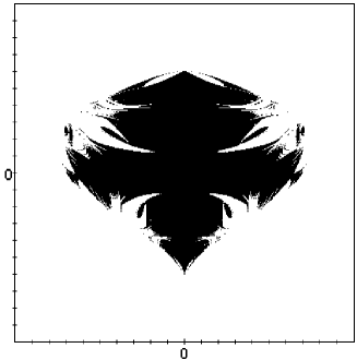
Figure 28: Bush B$[a^{4},i]$ in FPU-$\alpha$ with $N=8$.

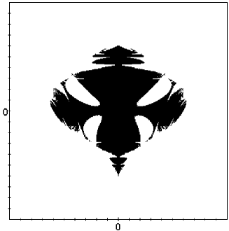
Figure 29: Bush B$[a^{4},i]$ in FPU-$\alpha$ with $N=12$.

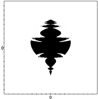
Figure 30: Bush B$[a^{4},i]$ in FPU-$\alpha$ with $N=16$.

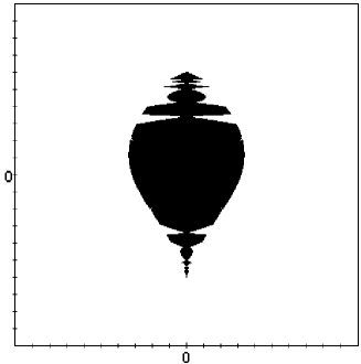
Figure 31: Bush B$[a^{4},i]$ in FPU-$\alpha$ with $N=20$.

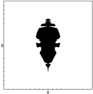
Figure 32: Bush B$[a^{4},i]$ in FPU-$\alpha$ with $N=24$.

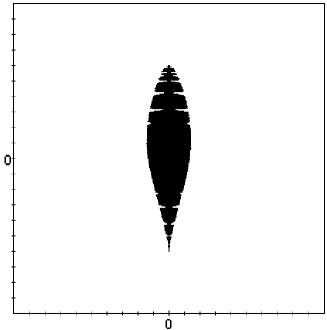
Figure 33: Bush B$[a^{4},i]$ in FPU-$\alpha$ with $N=48$.

Since we use similar stability diagrams for all one-dimensional bushes, let us describe their structure in more detail. In Fig. 7, each point $(A,k)$ determines a certain value of the root mode amplitude $A$ of the bush B$[\hat{a}^{2},\hat{i}]$ and a certain value $k=\frac{\pi j}{N}$, which is connected with the index $j$ of a fixed mode of the FPU-$\alpha$ chain. The black points $(A,k)$ correspond to the case where the mode $j=k\frac{N}{\pi}$ becomes excited because of its parametric interaction with the mode of the bush B$[\hat{a}^{2},\hat{i}]$. The white color denotes the opposite case: the corresponding mode $j$, being zero at the initial instant, continues to be zero in spite of its interaction with the considered bush. Dashed vertical lines correspond to the modes ($j=1,2,\dotsc,12$) for the FPU chain with $N=12$ particles. Considering stability diagrams, we must make one remark concerning normalization of the normal modes. In Eq. (17), there is the normalizing factor $\frac{1}{\sqrt{N}}$ which leads to the relation $\left|\bm{\psi}_{k}\right|^{2}=1$. Because of this factor, the absolute values of the individual atomic displacements corresponding to a given mode $\bm{\psi}_{k}$ tend to zero for $N\rightarrow\infty$. Such normalization of the normal modes is not convenient for studying the bush stability. Indeed, the critical value of atomic displacements, associated with the loss of stability, say, for the bush B$[\hat{a}^{2},\hat{i}]$ is equal to $x_{c}=0.30292/\alpha$ (this result can be easy obtained from Eq. (48) (see [1]). This value $x_{c}$ does not depend on the number $N$ of particles in the FPU chain. Because of this reason, depicting stability diagrams of one-dimensional and two-dimensional bushes in Figs. 28-33, we use different normalization of the normal modes than that in Eq. (17), namely, we simply reject the factor $\frac{1}{\sqrt{N}}$ which presents in Eq. (17). Then, the maximal value of the atomic displacements corresponding to every normal mode $\bm{\psi}_{k}$ turns out to be equal to $\sqrt{2}$.

We have just discussed the stability of the bush B$[\hat{a}^{2},\hat{i}]$. Now we intend to consider the stability of all the other one-dimensional bushes in the FPU-$\alpha$ and FPU-$\beta$ chains. There are three such bushes for every monoatomic nonlinear chain with dihedral symmetry group, but for the FPU-$\beta$ model, there exist three additional one-dimensional bushes because of the evenness of its potential [15]. For investigating stability of these bushes (three for the FPU-$\alpha$ chain and six for the FPU-$\beta$ chain), we shall also use the Floquet method.

There are two difficulties in implementing of this method for one-dimensional bushes in the general case, as compared to that for the above considered bush B$[\hat{a}^{2},\hat{i}]$. Indeed, the dynamical equations for the bushes B$[\hat{a}^{2},\hat{i}]$ and B$[\hat{a}^{4},\hat{a}\hat{i}]$ in the FPU-$\alpha$ model are reduced to the harmonic oscillator equation (with different frequencies), while the dynamical equations for all the other bushes turn out to be nonlinear. As a consequence, the period $T$ of the oscillations, described by the bush of such a type, depends on the amplitude $\mu_{0}$ of these oscillations ($T=T(\mu_{0})$). Therefore, we must construct the monodromy matrix by integration of the linearized dynamical equations, for the considered chain, over the period $T(\mu_{0})$. This period must be found for every value $\mu_{0}$ before obtaining the monodromy matrix.

The second difficulty is that the linearized dynamical system (near the appropriate exact solution to the given bush) can be split into the subsystems whose dimension (3 or 4) can be higher than that for the case of the bush B$[\hat{a}^{2},\hat{i}]$. As a result, we must deal, respectively, with $6\times 6$ or $8\times 8$ monodromy matrices.

5 Stability of one-dimensional bushes for the FPU chains

We will consider the stability of the bushes for the FPU-$\alpha$ and FPU-$\beta$ models separately.

5.1 FPU-$\alpha$ chain

The exact dynamical equations for the FPU-$\alpha$ chain in the modal space are given by Eqs. (39).

We want to linearize these equations in the vicinity of the solution described by a given one-dimensional bush. There are three one-dimensional bushes associated with the subgroups of the dihedral group of the monoatomic chains with the appropriate divisibility properties of the number $N$ of the particles (see Table 2): B$[\hat{a}^{2},\hat{i}]$ for $N\mod 2=0$, B$[\hat{a}^{3},\hat{i}]$ for $N\mod 3=0$, B$[\hat{a}^{4},\hat{a}\hat{i}]$ for $N\mod 4=0$. The following root modes correspond, respectively, to them: $\nu(t)\bm{\psi}_{N/2}$, $\nu(t)[\varepsilon_{1}\bm{\psi}_{N/3}+\varepsilon_{2}\bm{\psi}_{2N/3}]$, $\nu(t)[\bm{\psi}_{N/4}+\bm{\psi}_{3N/4}]$. Note that the root modes for the bushes B$[\hat{a}^{3},\hat{i}]$ and B$[\hat{a}^{4},\hat{a}\hat{i}]$ are the certain superpositions of the conjugate modes with time-independent coefficients $\left[\varepsilon_{1}=\sin\left(\frac{\pi}{12}\right),\varepsilon_{2}=\cos\left(\frac{\pi}{12}\right)\right]$.

Let us consider the bush B$[\hat{a}^{3},\hat{a}^{2}\hat{i}]$. Linearizing the FPU-$\alpha$ dynamical equations near the solutions $\bm{X}_{0}(t)=\nu(t)\varepsilon_{3}[\bm{\psi}_{N/3}-\bm{\psi}_{2N/3}]$ of this bush $\left[\varepsilon_{3}=\frac{\sqrt{2}}{2}\right]$, we must consider the amplitudes $\nu_{N/3}(t)=\varepsilon_{3}\nu(t)$ and $\nu_{2N/3}(t)=-\varepsilon_{3}\nu(t)$ in Eqs. (39) to be much greater than those of all other modes or, more precisely, $\nu_{j}(t)$ with $j\neq\frac{N}{3},\frac{2N}{3}$ must be treated as the infinitesimal values. Then we retain in Eqs. (39) only linear terms with respect to the modes $\nu_{j}(t)$ ($j\neq\frac{N}{3},\frac{2N}{3}$) which do not contribute to the given bush. The result of this computational procedure can be written as follows

$$\ddot{\nu}_{j}+\omega_{j}^{2}\nu_{j}=-\frac{\alpha\sqrt{6}}{\sqrt{N}}\nu(t) \left[\left(1+\sqrt{3}\sin\frac{2\pi j}{N}-\cos\frac{2\pi j}{N}\right)\nu_{\frac{N}{3}+j}+\right.$$ (49)

$$\;\left.\left(1-\sqrt{3}\sin\frac{2\pi j}{N}-\cos\frac{2\pi j}{N}\right)\nu_{\frac{2N}{3}+j}\right],$$

$$j=1,2,\cdots,N-1.$$

It can be easy seen from this form of linearized dynamical system that, for every fixed $j$, the modes $\nu_{j}$, $\nu_{N/3+j}$ and $\nu_{2N/3+j}$, being coupled by Eq. (49), are decoupled from all other modes. Therefore, we obtain for $j=1,2,\cdots,\frac{N}{3}-1$ the following $3\times 3$ systems of ordinary differential equations with periodic coefficients proportional to the function $\nu(t)$:

$$\begin{array}[]{l}\ddot{\nu}_{j}+\omega_{j}^{2}\nu_{j}=-\frac{\alpha\sqrt{6}}{\sqrt{N}}\nu(t)\left[{\left({1-2\cos\left({\frac{{2\pi j}}{N}+\frac{\pi}{3}}\right)}\right)\nu_{\frac{N}{3}+j}+\left({1-2\sin\left({\frac{{2\pi j}}{N}+\frac{\pi}{6}}\right)}\right)\nu_{\frac{{2N}}{3}+j}}\right],\\ \ddot{\nu}_{\frac{N}{3}+j}+\omega_{\frac{N}{3}+j}^{2}\nu_{\frac{N}{3}+j}=-\frac{\alpha\sqrt{6}}{\sqrt{N}}\nu(t)\left[{\left({1-2\cos\left({\frac{{2\pi j}}{N}+\frac{\pi}{3}}\right)}\right)\nu_{j}+\left({1+2\cos\frac{{2\pi j}}{N}}\right)\nu_{\frac{{2N}}{3}+j}}\right],\\ \ddot{\nu}_{\frac{2N}{3}+j}+\omega_{\frac{2N}{3}+j}^{2}\nu_{\frac{2N}{3}+j}=-\frac{\alpha\sqrt{6}}{\sqrt{N}}\nu(t)\left[{\left({1-2\sin\left({\frac{{2\pi j}}{N}+\frac{\pi}{6}}\right)}\right)\nu_{j}+\left({1+2\cos\frac{{2\pi j}}{N}}\right)\nu_{\frac{N}{3}+j}}\right].\\ \end{array}$$ (50)

In turn, the function $\nu(t)$ is the solution to the dynamical equation

$$\ddot{\nu}+3\nu=\frac{3\sqrt{6}}{2}\frac{\alpha}{\sqrt{N}}\nu^{2}$$

of the considered bush B$[\hat{a}^{3},\hat{a}^{2}\hat{i}]$. Thus, the stability of the bush B$[\hat{a}^{3},\hat{a}^{2}\hat{i}]$ can be investigated by the Floquet method applied to the systems (50) for $j=1,2,\cdots,\frac{N}{3}-1$.

Similarly to the above said, we can obtain the $4\times 4$ systems of differential equations for investigation of stability of the bush B$[\hat{a}^{4},\hat{a}\hat{i}]$. All systems of such a type, which must subjected to the further Floquet analysis, are given for the FPU-$\alpha$ chain in Table 8.

5.2 FPU-$\beta$ chain

We have obtained the linearized dynamical equations for one-dimensional bushes in the FPU-$\alpha$ chain by linearizing the exact nonlinear equations (39) defined in the modal space. This method, namely, obtaining the exact equations in the modal space with their subsequent linearization, is not the simplest method for our purpose. Indeed, we can, firstly, linearize the dynamical equations in the configuration space and only then transform the obtained equations to the modal space. In this manner, we can obtain the linearized equations in the modal space for different nonlinear chains, in particular, for the FPU-$\beta$ chain. Moreover, we want to find the dynamical equations linearized near the solution

$$\bm{X}_{0}(t)=\nu(t)\bm{c},$$ (51)

which describes the exact nonlinear regime corresponding to the considered one-dimensional bush. Here $\bm{c}$ is a constant vector which determines the directions of displacements of all particles in the chain, while $\nu(t)$ is a time-dependent function satisfied the dynamical equation of a given 1D bush

$$\ddot{\nu}+\omega^{2}\nu=F(\nu).$$ (52)

Here $F(\nu)$ is a certain nonlinear function.

Let us then suppose that

$$\bm{X}(t)=\bm{X}_{0}(t)+\bm{\delta}(t)$$ (53)

with $\bm{\delta}(t)=\left\{\delta_{1}(t),\cdots,\delta_{N}(t)\right\}$ being an infinitesimal vector, and substitute $\bm{X}(t)$ in this form into the dynamical equations of the nonlinear chain in the configuration space. For the chain with dynamical equations

$$\ddot{x}_{k}=(x_{k+1}+x_{k-1}-2x_{k})+\gamma\left[(x_{k+1}-x_{k})^{m}-(x_{k}-x_{k-1})^{m}\right],\quad k=1,2,\cdots,N,$$ (54)

and with periodic boundary conditions $x_{N+1}(t)=x_{1}(t)$, $x_{0}(t)=x_{N}(t)$, after linearization with respect to $\bm{\delta}(t)$, we obtain

$$\ddot{\bm{\delta}}=B(t)\bm{\delta}.$$ (55)

Here time-periodic matrix $B(t)$ is almost three-diagonal (see Fig. 6) and can be determined by the equations

$$\begin{array}[]{l}b_{j,j}=-2-\tilde{\gamma}(t)\left[(c_{j+1}-c_{j})^{m-1}+(c_{j}-c_{j-1})^{m-1}\right],\\ b_{j,j-1}=1+\tilde{\gamma}(t)(c_{j}-c_{j-1})^{m-1},\\ b_{j,j+1}=1+\tilde{\gamma}(t)(c_{j+1}-c_{j})^{m-1},\end{array}$$

where $\tilde{\gamma}(t)=\gamma m\nu^{m-1}(t)$.

*	*						*
*	*	*
	*	*	*
		*	*	*
			*	*	*
				*	*	*
					*	*	*
*						*	*

Figure 6: The structure of the matrix $B$ from Eq. 55 (for $N=8$).

The vector Eq. (55) represents the linearized dynamical equations of the considered chain (54) in the configuration space. Now, we must transform these equations to the modal space. Let

$$\bm{\delta}(t)=\sum_{j=1}^{N-1}\nu_{j}(t)\bm{\psi}_{j},$$ (56)

where the basis vectors $\bm{\psi}_{j}$ are determined by Eq. (17). Substituting $\bm{\delta}(t)$ from Eq. (56) into Eq. (55) and taking into account that these basis vectors are orthonormal, one can obtain the final dynamical equations of the chain, linearized near the solution (51) to a given one-dimensional bush. It must be noted, that this transformation, being simple in principle, is practically very cumbersome. We performed it with the aid of the mathematical packet MAPLE. The results of this procedure are listed for all one-dimensional bushes in the FPU-$\alpha$ and FPU-$\beta$ chains in Table 8 and Table 9, respectively.

As can be seen from Table 9, the full systems of linearized differential equations corresponding to different one-dimensional bushes in the FPU-$\beta$ chain split into certain subsystems whose dimensionalities are equal to $1$, $2$, $3$.

These systems contain time-periodic coefficients proportional to $\nu^{2}(t)$, where $\nu(t)$ is the solution to the Duffing equation

$$\ddot{\nu}+\omega^{2}\nu=\gamma\nu^{3}.$$

The coefficients $\omega^{2}$ and $\gamma$ are, naturally, different for different bushes.

Using Tables 8 and 9, we can investigate the stability of all one-dimensional bushes, with the aid of the Floquet method, for the FPU-$\alpha$ and FPU-$\beta$ models, respectively.

In our bush stability diagrams (see Figs. 7-15), we depict regions of stability (white color) and instability (black color) for individual modes $j=1,2,3,\dotsc,N-1$ of the FPU chains. The loss of stability by any mode, which does not belong to a given bush, leads to the loss of stability by the entire bush. The fact that we can study stability of individual modes allows us to investigate the bush stability not only for the chains with finite number of particles, but also for the case of thermodynamical (continuum) limit $N\rightarrow\infty$ (see a discussion in the next section).

Practically, we study the eigenvalues of the monodromy matrices for a certain subsets of sleeping modes. We choose as many points on the horizontal $k$-axis ($k=\frac{\pi j}{N}$), as it is necessary for obtaining sufficiently accurate picture. In some cases, the density of the analyzed $k$-points corresponds to $N\sim 10^{5}$. Usually, we recognize instability of a given set of sleeping modes, if there are eigenvalues of the corresponding monodromy matrix with modules exceeding $1$ by $10^{-5}$.

In Table 10, for the case $N=12$, we present the thresholds of the loss of stability for all one-dimensional bushes in the FPU-$\alpha$ and FPU-$\beta$ chains. In the stability diagrams (Figs. 7-15), all possible modes for this case ($j=1,2,3,\dotsc,12$) are depicted by vertical dashed lines. Using these diagrams, one can understand, in some sense, the cause of the given threshold values of bush stability for the FPU chains with $N=12$ (see below).

5.3 Diagrams of stability for one-dimensional bushes in the FPU-$\alpha$ chain

First of all, we would like to emphasize, that studying the stability of bushes of normal modes, we can restrict ourselves to only one specimen from the set of “dynamical domains” which represent equivalent bushes (see the previous section).

Now we consider the stability diagrams for the bushes in the FPU-$\alpha$ chain.

5.3.1 Bush B$[\hat{a}^{2},\hat{i}]$

The stability diagram for this bush (see Fig. 7) has already been discussed. Let us recall that in all our diagrams, for one-dimensional bushes, the stability regions are white, while unstable regions are black.

5.3.2 Bush B$[\hat{a}^{3},\hat{i}]$

In the configuration and modal spaces this bush looks, respectively, as follows:

$$\bm{X}(t)=\left\{x(t),0,-x(t)|x(t),0,-x(t)|\cdots\right\}=\nu(t)\left\{\varepsilon_{1}\bm{\psi}_{N/3}+\varepsilon_{2}\bm{\psi}_{2N/3}\right\}.$$ (57)

The stability diagram for the bush B$[\hat{a}^{3},\hat{i}]$ is presented in Fig. 8. The domain depicted in grey color corresponds to the disruption of the FPU-$\alpha$ chain (atoms escape from the potential wells in which the vibrational motion can occur). Thus, we must distinguish between the stability of the chain itself and the stability of a given vibrational regime, i.e., of a bush of modes, in this chain.

Let us imagine a horizontal line in Fig. 8 corresponding to a given value $A$ of the bush root mode. This line can partially pass through the white and partially through the black regions of the considered stability diagram. Actually, the parts of this line belonging to the black (unstable) region represent the set of modes which are excited because of the interactions with the bush root mode at the fixed level of its amplitude ($A$). If $A$ is very small, our horizontal line $A=const$ intersects the narrow unstable regions near the mode numbers $j=0,\frac{N}{3},\frac{2N}{3}$ and $N$.

Let us suppose that $N=12$ and $A<<1$. Then it is easy to see from Fig. 8 that only two modes, corresponding to $j=\frac{N}{3}$ and $j=\frac{2N}{3}$, are excited in our mechanical system. This fact is consistent with the stability of the bush B$[\hat{a}^{3},\hat{i}]$ for small values of its root mode amplitude. Indeed, according to Eq. (57), this bush contains only two (conjugate) modes $\nu_{N/3}(t)$ and $\nu_{2N/3}(t)$ with the certain relation between their amplitudes:

$$\nu_{N/3}(t)=\varepsilon_{1}\nu(t),\quad\nu_{2N/3}(t)=\varepsilon_{2}\nu(t)$$ (58)

Moreover, we can find the threshold of the stability loss of the bush B$[\hat{a}^{3},\hat{i}]$ directly from the diagram in Fig. 8, taking into account that all the possible modes for the case $N=12$ are marked by vertical dashed lines. This threshold is the minimal vertical distance from the horizontal coordinate axis to the black (unstable) region for $j=1,2,3,5,6,7,9,10,11$. The stability thresholds for all one-dimensional bushes in the FPU-$\alpha$ and FPU-$\beta$ chains for $N=12$ are given in Table 10. From this table, we find that the stability threshold for the bush B$[\hat{a}^{3},\hat{i}]$ (the critical value $x_{c}$ of the atomic displacements) is equal to $x_{c}=0.203$. The corresponding critical values of the root mode amplitude ($A_{c}$) and the energy ($E_{c}$) are equal to $A_{c}=0.166$, $E_{c}=0.047$.

Let us now increase the value $A$ of the root mode amplitude of the bush B$[\hat{a}^{3},\hat{i}]$. Such an increase leads to the broadening of the unstable regions near the $j=0,\frac{N}{3},\frac{2N}{3},N$ which intersects the line $A=const$ in Fig. 8. This fact does not affect the stability of the bush B$[\hat{a}^{3},\hat{i}]$ for $N=12$, as long as there are no modes $\nu_{j}$ with $j=1,2,\cdots,11$ (except the modes $\nu_{N/3}$ and $\nu_{2N/3}$) which fall into the above-mentioned broadening unstable intervals.

On the other hand, if $N\rightarrow\infty$ (continuum limit), the mode density, i.e. the density of vertical dashed lines in Fig. 8, increases and there appear narrow groups of modes near the values $j=0,\frac{N}{3},\frac{2N}{3},N$ ($k=0,\frac{\pi}{3},\frac{2\pi}{3},\pi$). This case corresponds to the onset of the modulation instability of the considered bush of modes. Note that we then have a bush of narrow wave packets which gradually collapses on a long time scale. Thus, we conclude that the bush B$[\hat{a}^{3},\hat{i}]$, being stable for small number of particles in the chain ($N$), for a fixed value of its root mode amplitude, becomes unstable in the continuum limit $N\rightarrow\infty$.

5.3.3 Bush B$[\hat{a}^{4},\hat{a}\hat{i}]$

The one-dimensional bush B$[\hat{a}^{4},\hat{a}\hat{i}]$ can be written as follows

$$\bm{X}(t)=\left\{0,x(t),0,-x(t)|0,x(t),0,-x(t)|\cdots\right\}=\frac{\sqrt{2}}{2}\nu(t)\left[\bm{\psi}_{N/4}+\bm{\psi}_{3N/4}\right].$$ (59)

Thus, it represents a superposition of two conjugate modes $\bm{\psi}_{N/4}$ and $\bm{\psi}_{3N/4}$ with equal amplitudes

$$\nu_{N/4}(t)=\nu_{3N/4}(t)=\frac{\sqrt{2}}{2}\nu(t).$$ (60)

According to the Table 10, the threshold of the stability loss for the bush B$[\hat{a}^{4},\hat{a}\hat{i}]$ in the FPU-$\alpha$ chain, in contrast to the similar thresholds for all other bushes, is equal to zero. In particular, the loss stability threshold (LST) for the same bush in the FPU-$\beta$ chain is equal to $1.161$ (for the case $N=12$). Let us discuss this unusual case in more detail.

In Fig. 9, we see that besides the modes $\nu_{N/4}(t)$ and $\nu_{3N/4}(t)$ contributing to B$[\hat{a}^{4},\hat{a}\hat{i}]$, the mode $\nu_{N/2}(t)$ is also excited for arbitrarily small values of the root mode amplitude of the considered bush. On the other hand, all the results presented in Table 10 and in Figs. 7-15 are obtained numerically by the Floquet method and, partially, by a straightforward integration of the dynamical equations of the FPU-chains. Since numerical results are only approximate, it is desirable to prove analytically that the LST for the bush B$[\hat{a}^{4},\hat{a}\hat{i}]$ in the FPU-$\alpha$ chain is indeed equal to zero exactly.

In the general case, the presence of three modes $\nu_{N/4}(t)$, $\nu_{N/2}(t)$, $\nu_{3N/4}(t)$, in the dynamical regime, means that we have the three-dimensional bush B$[\hat{a}^{4}]$ (see [17]) with

$$\bm{X}(t)=\nu_{N/4}(t)\bm{\psi}_{N/4}+\nu_{N/2}(t)\bm{\psi}_{N/2}+\nu_{3N/4}(t)\bm{\psi}_{3N/4}.$$ (61)

Therefore, one can suppose that the initially excited one-dimensional bush B$[\hat{a}^{4},\hat{a}\hat{i}]$ transforms spontaneously into the three-dimensional bush B$[\hat{a}^{4}]$:

$$\text{B}[\hat{a}^{4},\hat{a}\hat{i}]\rightarrow\text{B}[\hat{a}^{4}].$$ (62)

This transformation is accompanied by the lowering of the symmetry, because of the loss of the invertion element $\hat{a}\hat{i}$. In the dynamical picture of the above transformation, the new mode $\nu_{N/2}(t)$ appears and the specific relation between the modes $\nu_{N/4}(t)$ and $\nu_{3N/4}(t)$, presented in the bush B$[\hat{a}^{4},\hat{a}\hat{i}]$, is destroyed:

$$\nu_{N/4}(t)\neq\nu_{3N/4}(t).$$

Thus, we must now prove that the bush B$[\hat{a}^{4},\hat{a}\hat{i}]$ loses its stability with respect to the interaction exactly with the mode $\nu_{N/2}$. So, let us exclude all the other modes of the FPU-$\alpha$ chain from our consideration and focus only on the transformation (62). Obviously, if we prove that the stability threshold of the bush B$[\hat{a}^{4},\hat{a}\hat{i}]$, for the transformation (62), is zero, then it is also zero with respect to the interactions with all modes of the chain.

Because of the above said, let us consider the dynamical equations of the three-dimensional bush B$[\hat{a}^{4}]$ which can be written as follows

$$\begin{array}[]{l}\ddot{\mu}_{1}+2\mu_{1}=-\frac{8\alpha}{N}\mu_{1}\mu_{2},\\ \ddot{\mu}_{2}+4\mu_{2}=-\frac{4\alpha}{N}\left(\mu_{1}^{2}-\mu_{3}^{2}\right),\\ \ddot{\mu}_{3}+2\mu_{3}=\frac{8\alpha}{N}\mu_{2}\mu_{3}.\end{array}$$ (63)

Here we renamed the modes $\nu_{N/4}(t)$, $\nu_{N/2}(t)$ and $\nu_{3N/4}(t)$ as $\mu_{1}(t)$, $\mu_{2}(t)$ and $\mu_{3}(t)$, respectively.

In the dynamical regime corresponding to the bush B$[\hat{a}^{4},\hat{a}\hat{i}]$ only one degree of freedom is excited (see Eq. (59)). In our new notation it can be written as

$$\bm{X}(t)=\mu_{1}(t)\bm{\psi}_{N/4}+\mu_{3}(t)\bm{\psi}_{3N/4},$$ (64)

where $\mu_{1}(t)=\mu_{3}(t)$. Substituting $\mu_{1}(t)=\mu_{3}(t)$, $\mu_{2}(t)=0$ into Eqs. (63), we find that the first and third equations are both reduced to the equation of the harmonic oscillator

$$\ddot{\mu}_{1}+2\mu_{1}=0,$$ (65)

while both sides of the second equation turn out to be zero. Thus,

$$\mu_{1}^{(0)}(t)=A\cos(\sqrt{2}t+\phi_{0})$$ (66)

and we can linearize Eqs. (63) near the dynamical regime (66). Note that one can assume $\phi_{0}=0$ in Eq. (66), without loss of generality, since it is possible to shift the time variable $t$ in the dynamical equations of the bush B$[\hat{a}^{4}]$ by the appropriate value.

According to the general idea of linearization, let us suppose that

$$\begin{array}[]{lll}\mu_{1}(t)&=&\mu_{1}^{(0)}(t)+\delta_{1}(t),\\ \mu_{2}(t)&=&\delta_{2}(t),\\ \mu_{3}(t)&=&\mu_{1}^{(0)}(t)+\delta_{3}(t).\end{array}$$ (67)

Here $\delta_{i}$ ($i=1,2,3$) are small corrections to the original dynamical regime (64) $\left\{\mu_{1}^{(0)}(t),0,\mu_{1}^{(0)}(t)\right\}$ which is determined by the one-dimensional bush B$[\hat{a}^{4},\hat{a}\hat{i}]$. Let us now substitute (67) into Eqs. (63) and neglect all nonlinear in $\delta_{i}$ terms. Then we have:

$$\begin{array}[]{lll}\ddot{\delta}_{1}+2\delta_{1}&=&-8\alpha A\cos(\sqrt{2}t)\delta_{2},\\ \ddot{\delta}_{2}+4\delta_{2}&=&-8\alpha A\cos(\sqrt{2}t)(\delta_{1}-\delta_{3}),\\ \ddot{\delta}_{3}+2\delta_{3}&=&8\alpha A\cos(\sqrt{2}t)\delta_{2}.\end{array}$$ (68)

Subtracting the third equation from the first equation and introducing new variables $\gamma_{1}(t)=\delta_{1}(t)-\delta_{3}(t)$, $\gamma_{2}(t)=\delta_{2}(t)$, we obtain finally

$$\begin{array}[]{lcl}\ddot{\gamma}_{1}+2\gamma_{1}&=&-16\alpha A\cos(\sqrt{2}t)\gamma_{2},\\ \ddot{\gamma}_{2}+4\gamma_{2}&=&-8\alpha A\cos(\sqrt{2}t)\gamma_{1}.\end{array}$$ (69)

Namely for these equations, we must find analytically the nontrivial solution ($\gamma_{1}(t)\neq 0$, $\gamma_{2}(t)\neq 0$)

Note that the same system can be obtained from the linearized equations for investigation of the stability of the bush B$[\hat{a}^{4},\hat{a}^{3}\hat{i}]$ which is presented in Table 8 for the FPU-$\alpha$ chain. Indeed, let us assume $j=0$ in the last system from this table, keeping in mind the relation $k=\frac{\pi j}{N}$. Then we have

$$\begin{array}[]{lllll}\ddot{\nu}_{0}&&&=&0,\\ \ddot{\nu}_{N/4}&+&\omega_{N/4}^{2}\nu_{N/4}&=&-\frac{4\sqrt{2}\alpha}{\sqrt{N}}\mu(t)\nu_{N/2}(t),\\ \ddot{\nu}_{N/2}&+&\omega_{N/2}^{2}\nu_{N/2}&=&-\frac{4\sqrt{2}\alpha}{\sqrt{N}}\mu(t)\left[\nu_{N/4}(t)+\nu_{3N/4}(t)\right],\\ \ddot{\nu}_{3N/4}&+&\omega_{3N/4}^{2}\nu_{3N/4}&=&-\frac{4\sqrt{2}\alpha}{\sqrt{N}}\mu(t)\nu_{N/2}(t),\end{array}$$ (70)

where $\omega_{j}^{2}=4\sin^{2}(\frac{\pi j}{N})$, while $\mu(t)=A\cos(\sqrt{2}t)$ is the solution to the equation $\ddot{\mu}+2\mu=0$. Summing the second and forth equations of the system (70) leads us again to Eqs. (69), where $\gamma_{1}(t)=\nu_{N/4}(t)+\nu_{3N/4}(t)$, $\gamma_{2}(t)=\nu_{N/2}(t)$.

Thus, the analysis of the stability loss by the bush B$[\hat{a}^{4},\hat{a}\hat{i}]$ is reduced to the problem of parametric excitation of the nontrivial solution to Eqs. (69). On the other hand, it is well known that the onset of unstable motion for the Mathieu equation can be investigated with the aid of different asymptotic methods of nonlinear mechanics (averaging method, multiscale method, etc.). In [20], we use one of such a type methods, namely, the normalization procedure based on the Poincare-Dulac theorem, for studying the parametric excitation in the system (69). Using this procedure, we remove, step by step, the so-called nonresonance terms of a given order to higher orders in the small parameter (in our case, this is the root mode amplitude $A$) with the aid of the appropriate nonlinear transformations of the dynamical variables $\gamma_{i}(t)$. In such a way, the normalized system of differential equations with respect to new variables $\tilde{\gamma}_{i}(t)$ is obtained and, as a rule, this system turns out to be simpler than the original system.

In [20], it was shown that the normalized equations up to $O(A^{3})$, obtained from Eqs. (69), can be solved exactly. The corresponding solution for $\tilde{\gamma}_{1}(t)$ contains the growing exponent $\exp(\sqrt{2}\alpha^{2}A^{2}t)$ which increases from zero for the arbitrary small value of the root mode amplitude $A$. For the old variable $\gamma_{1}(t)$ this exponent, being decomposed into the power series with respect to $A$, produces the unremovable secular term of the form

$$\alpha^{2}A^{2}\sqrt{2}t\sin(\sqrt{2}t+\delta).$$

From the above said, it is clear that the parametric excitation in the system (69) takes place for the arbitrary small value of the root mode amplitude $A$ and, therefore, the bush B$[\hat{a}^{4},\hat{a}\hat{i}]$ possesses the stability domain of zero size, as it has already been concluded directly from Fig. 9.

5.4 Diagrams of stability for one-dimensional bushes in the FPU-$\beta$ chain

5.4.1 Bush B$[\hat{a}^{2},\hat{i}]$

The stability diagram corresponding to the bush B$[\hat{a}^{2},\hat{i}]$ in the FPU-$\beta$ chain is presented in Fig. 10. From this diagram, one can see that for any finite $N$ and for sufficiently small root mode amplitude $A$, there exists, in our mechanical systems, only one mode $\nu_{N/2}(t)$, which is the root (and single!) mode of the bush B$[\hat{a}^{2},\hat{i}]$. On the other hand, if we fix arbitrary small value of $A$ and then begin to increase the number of particles $N$, such $N$ can be always found for which some other modes, close to the mode $\nu_{N/2}(t)$, turn out to be excited (see the center of the diagram 10). In other words, the threshold of the loss of stability of the considered bush decreases with increasing $N$. Thus, the bush B$[\hat{a}^{2},\hat{i}]$ becomes unstable in the continuum limit $N\rightarrow\infty$.

Another interesting fact can be revealed with the aid of the diagram 10. Namely, there are certain intervals of mode numbers on r.h.s. and l.h.s. of this diagram which cannot be excited because of the interactions with the mode $\nu_{N/2}(t)$. Note that the both above mentioned facts were found and discussed, in rather different terms, in the paper [14].

5.4.2 Bush B$[\hat{a}^{3},\hat{i}]$

The form of the bush B$[\hat{a}^{3},\hat{i}]$ in the configuration and modal spaces was given in Eq. (57) The corresponding stability diagram is shown in Fig. 11. From this diagram, we find that, for small amplitudes, the bush B$[\hat{a}^{3},\hat{i}]$ is not stable in the continuum limit $N\rightarrow\infty$, but can be stable for finite $N$. For example, for $N=12$ the stability takes place up to the value $A_{1}$ of the root mode amplitude $A$. Note that three horizontal dashed lines are depicted in Fig. 11: the lower line is described by the equation $A=A_{1}$, while the middle and upper lines correspond to the equations $A=A_{2}$ and $A=A_{3}$, respectively.

For $A_{1}<A<A_{2}$ all the modes, with the only exception of the modes with $j=\frac{2N}{12}=\frac{N}{6}$, $j=\frac{6N}{12}=\frac{N}{2}$ and $j=\frac{10N}{12}=\frac{5N}{6}$, are excited. Therefore, for $N=12$, the bush with trivial symmetry is excited. Indeed, the excitation of the mode with $j=\frac{N}{12}$ can lead, in principle, to excitation of all the modes with $j=\frac{kN}{12}$ ($k=1,2,\cdots,11$).

It is very interesting that there exists also the upper value ($A_{3}$) for the loss of stability of the bush B$[\hat{a}^{3},\hat{i}]$. Indeed, for $A>A_{3}$ (see Fig. 11) this bush turns out to be stable for all values of the number ($N$) of particles in the chain. Thus, the bush B$[\hat{a}^{3},\hat{i}]$ becomes stable even in the continuum limit, for such values of the root mode amplitude $A$.

5.4.3 Bush B$[\hat{a}^{4},\hat{a}\hat{i}]$

The description of the bush B$[\hat{a}^{4},\hat{a}\hat{i}]$ in the configuration and modal spaces has already been given by Eq. (59):

$$\bm{X}(t)=\left\{0,x,0,-x|0,x,0,-x|\dots\right\}=\varepsilon_{3}\nu(t)\left[\bm{\psi}_{N/4}+\bm{\psi}_{3N/4}\right].$$

The stability diagram for this bush for the FPU-$\beta$ chain is represented in Fig. 12. From this diagram, one can see that, for any finite $N$, the bush B$[\hat{a}^{4},\hat{a}\hat{i}]$ is stable for sufficiently small root mode amplitudes $A$. For example, for $N=12$, this bush loses its stability only for $A>A_{1}$ (see Fig. 12). For very large $N$, the bush B$[\hat{a}^{4},\hat{a}\hat{i}]$ practically also remains stable for sufficiently small $A$ because the intervals of the numbers of the excited modes turn out to be very narrow (these intervals are situated near $j=\frac{N}{4}$ and $j=\frac{3N}{4}$). In the continuum limit $N\rightarrow\infty$, rigorously speaking, the bush B$[\hat{a}^{4},\hat{a}\hat{i}]$ appears to be unstable, but its instability is weak.

We have just discussed the stability of all one-dimensional bushes for the FPU-$\beta$ chain which are induced by the dihedral symmetry group. Now let us consider the stability of three “additional” one-dimensional bushes whose existence is brought about by the evenness of the potential of the FPU-$\beta$ chain.

5.4.4 Bush B$[\hat{a}^{3},\hat{i}\hat{u}]$

The description of this bush in configuration and modal spaces looks as follows:

$$\bm{X}(t)=\left\{x,-2x,x|x,-2x,x|\dots\right\}=\nu(t)\left[\varepsilon_{2}\bm{\psi}_{N/3}-\varepsilon_{1}\bm{\psi}_{2N/3}\right].$$ (71)

The stability diagram of the bush B$[\hat{a}^{3},\hat{i}\hat{u}]$ is given in Fig. 13. It seems similar to that of the above discussed bush B$[\hat{a}^{3},\hat{i}]$ (see Fig. 11). Therefore, the discussion of the stability properties of the bush B$[\hat{a}^{3},\hat{i}\hat{u}]$ can be practically reduced to that of the bush B$[\hat{a}^{3},\hat{i}]$.

5.4.5 Bush B$[\hat{a}^{4},\hat{i}\hat{u}]$

This bush can be described by the equation

$$\bm{X}(t)=\left\{x,-x,-x,x|x,-x,-x,x|\dots\right\}=\nu(t)\bm{\psi}_{N/4}.$$ (72)

The corresponding stability diagram is represented in Fig. 14 and looks as “rabbit ears”. For root mode amplitudes $A>A_{1}$ (see Fig. 14) this bush is stable for arbitrary $N$. It is interesting that for the case $N=12$ there are no excited modes, certainly, besides the mode $\bm{\psi}_{N/4}$ (or the mode $\bm{\psi}_{3N/4}$ for the equivalent bush B$[\hat{a}^{4},\hat{a}^{2}\hat{i}\hat{u}]$ which looks in the modal space as $\bm{X}(t)=\nu(t)\bm{\psi}_{3N/4}$). This is in agreement with Table 10 from which we find that this bush is stable, at least, up to the root mode amplitude $A<20$.

5.4.6 Bush B$[\hat{a}^{6},\hat{a}\hat{i},\hat{a}^{3}\hat{u}]$

This bush can be described as follows:

$$\bm{X}(t)=\left\{0,x,x,0,-x,-x|0,x,x,0,-x,-x|\dots\right\}=\nu(t)\left[\varepsilon_{1}\bm{\psi}_{N/6}+\varepsilon_{2}\bm{\psi}_{5N/6}\right].$$ (73)

One of the distinguishing features of the stability diagram for this bush (see Fig. 15) is the presence of three white regions in the “black sea” of instability. They correspond to the second stability zones for some modes whose numbers fall into these white regions. Another interesting feature of the stability diagram for the considered bush is the very narrow unstable intervals in the “white sea” of stability (see the black lines which resemble parabolas). We did not examine these unstable parabolas in detail, because they seem to be not very essential for consideration of the stability of the bush B$[\hat{a}^{6},\hat{a}\hat{i},\hat{a}^{3}\hat{u}]$. Indeed, they represent too narrow regions of unstable movements.

5.5 About numerical values of root mode amplitudes for the FPU chains

The FPU models of $\alpha$ and $\beta$ type, considered as exact mechanical systems, do not contain the interparticle distance $a$. As a consequence, one cannot estimate the reasonable values of the root mode amplitudes for the above discussed bushes. This is an important problem because atomic displacements in real crystals cannot, as a rule, exceed $10-15\%$ of the equilibrium interparticle distance.

On the other hand, we can consider FPU system as a certain approximation to more realistic models of one-dimensional crystals. Let us consider a nonlinear monoatomic chain with the Lennard-Jones potential $U(r)$ describing the interaction between the nearest particles:

$$U(r)=\varepsilon\left[\left(\frac{\sigma}{r}\right)^{12}-\left(\frac{\sigma}{r}\right)^{6}\right].$$ (74)

Here, $r$ is the interparticle distance, while $\varepsilon$ and $\sigma$ are certain constants.

Let us expand the force $f(r)$ acting on one particle, in Taylor series near the equilibrium interparticle distance $a=\sigma\sqrt[6]{2}$ up to the terms of the second order:

$$f(r)=-\frac{9\sqrt[3]{4}}{\sigma^{2}}(r-a)+\frac{189\sqrt{2}}{2\sigma^{3}}(r-a)^{2}.$$ (75)

Then we can write the Newton equations of motion in the form

$$m\ddot{x}_{i}=\frac{9\sqrt[3]{4}\varepsilon}{\sigma^{2}}\left(-2x_{i}+x_{i+1}+x_{i-1}\right)+\frac{189\sqrt{2}\varepsilon}{2\sigma^{3}}\left[\left(x_{i+1}-x_{i}\right)^{2}-\left(x_{i}-x_{i-1}\right)^{2}\right],$$ (76)

where $m$ is the mass of one particle.

Introducing new dimensionless time and space variables

$$t^{\prime}=\sqrt{\frac{9\sqrt[3]{4}\varepsilon}{m\sigma^{2}}}t,\quad x^{\prime}_{n}=\frac{21\sqrt[3]{2}}{a}x_{n},$$ (77)

we obtain the following equations:

$$\ddot{x}^{\prime}_{i}=(-2x^{\prime}_{i}+x^{\prime}_{i+1}+x^{\prime}_{i-1})+[(x^{\prime}_{i+1}-x^{\prime}_{i})^{2}-(x^{\prime}_{i}-x^{\prime}_{i-1})^{2}].$$ (78)

These equations precisely correspond to the FPU-$\alpha$ model considered in the present paper.

On the other hand, the dimensionless variables $x^{\prime}_{i}$, according to Eq. (77), are proportional to the ratio of the real atomic displacements $x_{i}$ and the equilibrium interparticle distance $a$. As it has already been noted, for real crystal, $x_{i}/a$ must not exceed $10-15\%$. The dimensionless displacements $x^{\prime}_{i}$ from the FPU-$\alpha$ model (78) can be considerably larger than this value, because of the coefficient $21\sqrt[3]{2}\approx 29.7$ before $x_{i}/a$. For example, if $x_{i}\sim 0.1a$, then $x^{\prime}_{i}\sim 3$.

Let us now recall that, studying the bush stability, we use such normalization of the normal modes, that their amplitudes are of the same order as the atomic displacements corresponding to them. Thus, the root mode amplitudes $A$ at about $3$ seem to be rather reasonable. It is precisely because of this fact that we depict the bush stability diagram up to $A$ of such an order of magnitude.

6 Stability of two-dimensional bushes for the FPU chains

In the previous section, we considered the stability of one-dimensional bushes with respect to increasing their root mode amplitudes. Such an increasing leads to strengthening of the parametric interactions of the root mode of a given bush with all the other modes which do not belong to this bush and, finally, to a loss of its stability. Actually, the threshold of the loss of stability of any one-dimensional bush depends only on its total energy (the energy of the initial excitation), but not on the distribution of this energy between the kinetic and potential counterparts [20]. In two last columns of Table 10 we give the energy thresholds of the loss of stability for all one-dimensional bushes in the FPU chains. In contrast to one-dimensional bushes, the stability of the multi-dimensional bushes depends not only on the energy of the initial excitation, but also on the complete set of the initial conditions. Let us consider this problem in more detail.

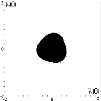
Figure 18: Stability diagram for the bush B$[a^{3}]$ in the FPU-$\alpha$ chain.

The four-dimensional phase space corresponds to the two-dimensional bushes considered below in the present paper. In Fig. 18-27, we depict only certain planar sections of the four-dimensional stability domains, aiming to show how nontrivial the boundary of these domains can be.

The complete set of initial conditions for the dynamical equations of a given two-dimensional bush determines the concrete values of $\nu_{1}(0),\dot{\nu}_{1}(0),\nu_{2}(0),\dot{\nu}_{2}(0)$, where $\nu_{i}(t)$ and $\dot{\nu}_{i}(t)$ ($i=1,2$) are the two modes of the considered bush and their velocities, respectively. We depict the bush stability diagrams (see Fig. 18-33) in certain planes which are chosen by fixing two of the four above-mentioned initial values. Most frequently, we specify $\dot{\nu}_{1}(0)=0,\dot{\nu}_{2}(0)=0$ and change $\nu_{1}(0),\nu_{2}(0)$ in some intervals near their zero values. Therefore, the initial kinetic energy assumed to be equal to zero and the dependence of bush stability on the initial mode amplitudes $\nu_{1}(0)$ and $\nu_{2}(0)$ is studied.

The diagrams discussed in the previous section allow us to analyze stability of one-dimensional bushes for the FPU chains with arbitrary number ($N$) of particles. Unfortunately, we cannot obtain similar diagrams for two-dimensional bushes. Stability diagrams considered in this section depend on the number of particles and, therefore, they must be constructed individually for each specific $N$. Because of this reason, we consider stability of 2D bushes only for fixed $N$ (for the most diagrams $N=12$). As a consequence, we do not discuss the stability properties of the 2D bushes with translation symmetry $[\hat{a}^{5}]$, $[\hat{a}^{8}]$ and $[\hat{a}^{10}]$ (the complete list of 2D bushes for the FPU chains can be found in Appendix).

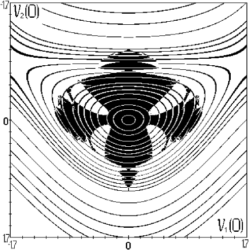
Figure 16: Stability diagram of the bush B$[a^{4},i]$ in the FPU-$\alpha$ chain with $N=12$ for the case $\dot{\nu}_{1}(0)=0$, $\dot{\nu}_{2}(0)=0$.

Firstly, let us consider the stability of the two-dimensional bush B$[\hat{a}^{4},\hat{i}]$ in the FPU-$\alpha$ chain with $N=12$ particles. The stability domain for this bush, in the plane of the initial values of its both modes $[\nu_{1}(0),\nu_{2}(0)]$, is presented in black color in the center of Fig. 16. This domain, resembling a beetle, is depicted on the background of the energy level lines. The bush B$[\hat{a}^{4},\hat{i}]$ loses its stability when we cross the boundary of the black region in any direction. Moreover, it can be shown that the considered bush transforms into different bushes of larger dimensions at different points of the boundary. Which bushes appear near the various parts of the boundary of the stability domain of the bush B$[\hat{a}^{4},\hat{i}]$ will be discussed elsewhere. Now we merely want to emphasize that the loss of stability of this bush is not determined only by the energy of the initial excitation (the boundary of stability domain does not coincide with any energy level line!), but depends on the relation between the values of its both modes $[\nu_{1}(0),\nu_{2}(0)]$, as well. Thus, the stability domain of the bush B$[\hat{a}^{4},\hat{i}]$ is strongly anisotropic: the linear size of this domain in different directions, from zero point $\nu_{1}(0)=0,\nu_{2}(0)=0$, turns out to be different.

The stability diagram of the bush B$[\hat{a}^{4},\hat{i}]$ in the FPU-$\alpha$ chain, depicted in Fig. 16, was obtained by the direct numerical experiment for the case $\dot{\nu}_{1}(0)=0,\dot{\nu}_{2}(0)=0$. Therefore, initial kinetic energy was equal to zero and the total excitation energy was purely potential.

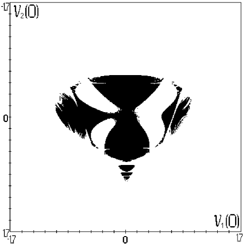
Figure 17: Stability diagram of the bush B$[a^{4},i]$ in the FPU-$\alpha$ chain with $N=12$ for the case $\dot{\nu}_{1}(0)=0.2$, $\dot{\nu}_{2}(0)=0.1$.

It is interesting to consider the case where the excitation energy is distributed at the initial instant, in some a manner, between its kinetic and potential counterparts. The appropriate stability diagram is depicted in Fig. 17. Actually, this is simply another section of the same four-dimensional stability domain of the considered bush which is determined by the equations $\dot{\nu}_{1}(0)=0.2,\dot{\nu}_{2}(0)=0.1$.

Comparing Fig. 16 and Fig. 17, one can see the effect of the “wind blowing from the right to the left”. This effect leads to a loss of the symmetry of the diagram in Fig. 16 with respect to the vertical axis passing through the origin.

Thus, the threshold of the loss of stability of the bush B$[\hat{a}^{4},\hat{i}]$ in the FPU-$\alpha$ chain depend essentially not only on the distribution of the initial energy between its two modes, but also between the kinetic and potential counterparts. Let us repeat, once more, that instead of dealing with the four-dimensional stability diagram, we investigate different sections of this domain.

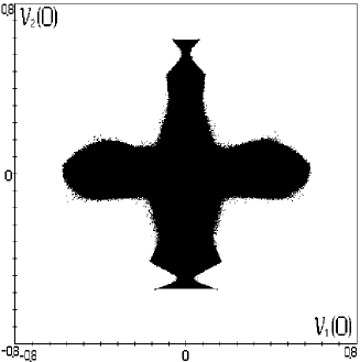
Figure 20: Stability diagram for the bush B$[a^{6},ai]$ in the FPU-$\alpha$ chain.

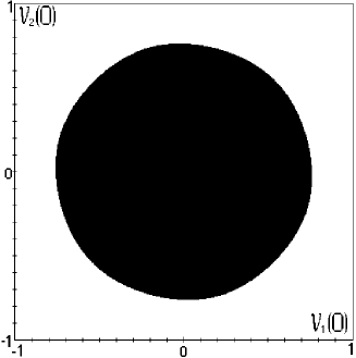
Figure 21: Stability diagram for the bush B$[a^{3}]$ in the FPU-$\beta$ chain.

The stability diagrams for two other two-dimensional bushes, B$[\hat{a}^{3}]$ and B$[\hat{a}^{6},\hat{a}\hat{i}]$, in the FPU-$\alpha$ chain are depicted in Fig. 18 and Fig. 20, respectively. These diagrams, as well as the diagrams in Fig. 21-27 for the FPU-$\beta$ chain, correspond to the initial conditions $\dot{\nu}_{1}(0)=0$, $\dot{\nu}_{2}(0)=0$, i.e. the kinetic energy of the initial excitation is supposed to be equal to zero.

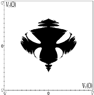
Figure 19: Stability diagram for the bush B$[a^{4},i]$ in the FPU-$\alpha$ chain.

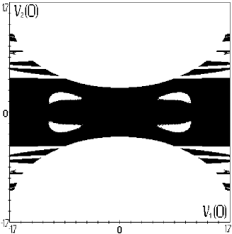
Figure 22: Stability diagram for the bush B$[a^{4},i]$ in the FPU-$\beta$ chain.

Let us emphasize that the stability diagrams for the same bushes in the FPU-$\alpha$ and FPU-$\beta$ chains look very different. As an example, one can compare Fig. 19 and Fig. 22 for the bush B$[\hat{a}^{4},\hat{i}]$ in FPU-$\alpha$ and FPU-$\beta$ chains, respectively. It is interesting to note that the last diagram (Fig. 22) demonstrates the presence of several regions of instability (white color) in the stable sea (black color).

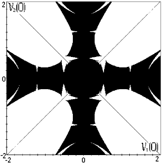
Figure 24: Stability diagram for the bush B$[a^{4},a^{2}u]$ in the FPU-$\beta$ chain.

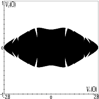
Figure 25: Stability diagram for the bush B$[a^{4},aiu]$ in the FPU-$\beta$ chain.

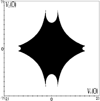
Figure 26: Stability diagram for the bush B$[a^{6},iu]$ in the FPU-$\beta$ chain.

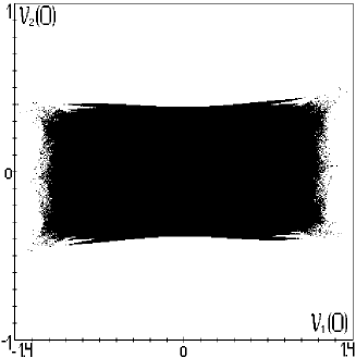
Figure 27: Stability diagram for the bush B$[a^{6},i,a^{3}u]$ in the FPU-$\beta$ chain.

In Figs. 24-27, we represent the stability diagrams corresponding to four additional two-dimensional bushes for the FPU-$\beta$ chain (as it has already been said, they are induced by the evenness of the potential of this model).

The most nontrivial picture corresponds to the stability diagram of the bush B$[\hat{a}^{4},\hat{a}^{2}\hat{u}]$. It resembles a chivalrous cross with two crossed swords (along the diagonals of the diagram). Note that these swords describe, actually, the stability of two equivalent one-dimensional bushes $\nu(t)[\bm{\psi}_{3}+\bm{\psi}_{9}]$ and $\nu(t)[\bm{\psi}_{3}-\bm{\psi}_{9}]$, while the two-dimensional bush B$[\hat{a}^{4},\hat{a}^{2}\hat{u}]$ is $\nu_{1}(t)\bm{\psi}_{3}+\nu_{2}(t)\bm{\psi}_{9}$.

For many bushes, the stability domains depend essentially on the number $N$ of particles in the chain. The area of the corresponding regions of stability, in our diagrams, tends often to decrease with the increasing of $N$. We demonstrate such a behavior in the cases $N=8,12,16,20,24,48$ for the bush B$[\hat{a}^{4},\hat{i}]$ in the FPU-$\alpha$ chain (see Figs. 28-33). Note that the stability domain of this bush shrinks only along the horizontal axis $\nu_{1}(0)$ when $N\rightarrow\infty$. This is the consequence of the fact that when $\nu_{1}(t)\rightarrow 0$ the bush B$[\hat{a}^{4},\hat{i}]=\nu_{1}(t)\bm{\psi}_{3N/4}-\nu_{2}(t)\bm{\psi}_{N/2}$ (or its equivalent form B$[\hat{a}^{4},\hat{a}^{2}\hat{i}]=\nu_{1}(t)\bm{\psi}_{N/4}+\nu_{2}(t)\bm{\psi}_{N/2}$) tends to the one-dimensional bush B$[\hat{a}^{2},\hat{i}]=\nu_{2}(t)\bm{\psi}_{N/2}$. On the other hand, the latter bush possesses, for $N\rightarrow\infty$, a finite one-dimensional interval of stability with respect to increasing of the initial value $\nu_{2}(0)$ of its single mode $\nu_{2}(t)$.

7 Conclusion

The bushes of normal modes as exact nonlinear excitations in the physical systems with discrete (point or space) symmetry groups were introduced and discussed in our previous papers [2, 3, 4, 6, 9, 10, 11]. In general case, bushes can be rather complex, for example, the bushes in the $C_{60}$ fullerene structure [11].

In [1], we considered bushes in monoatomic nonlinear chains which represent the simplest systems with translational symmetry. Mainly, we studied there the bushes induced by the group $T$ of pure translations and discussed only in part those induced by the dihedral symmetry group $D$. The stability of a few simplest bushes was also studied in [1]. Nevertheless, there are some more one-dimensional and two-dimensional bushes in the FPU-chains, in particular, those obtained by Bob Rink in [15], whose stability still has not been investigated. On the other hand, the problem of the bush stability is one of the most important problems in the general theory of the bushes of normal modes. Because of this, in the present paper, we discuss in detail the stability of all one-dimensional and some two-dimensional bushes in both FPU-$\alpha$ and FPU-$\beta$ chains.

Let us summarize the results obtained in the previous sections of this paper.

1. A simple crystallographic method for finding bushes in nonlinear chains is developed.

2. The stability of all one-dimensional bushes in the FPU-$\alpha$ (three bushes) and in the FPU-$\beta$ (six bushes, including those obtained in [15]) are investigated. The stability diagrams which can be used for studying stability of one-dimensional bushes for the FPU chains with any finite and infinite number of particles (continuum limit $N\rightarrow\infty$) are presented. They were obtained by Floquet method.

3. The stability diagrams of different type, which represent certain sections of four-dimensional stability domains, corresponding to some two-dimensional bushes in the FPU-$\alpha$ (three bushes) and in the FPU-$\beta$ (seven bushes), are found. These diagrams demonstrate explicitly that the bush stability domains depend not only on the energy of the initial excitation, but on the complete set of the initial conditions in the bush phase space.

The above mentioned diagrams for one-dimensional and two-dimensional bushes show how nontrivial the shape of the stability domains for the bushes of normal modes can be.

In this paper, we consider only the main mechanism for the loss of bush stability, wherein it is brought about by the parametric excitations of the bush modes with those modes which do not belong to the given bush. Nevertheless, one can consider some different reasons for a bush to lose its stability, such as a finite temperature of the thermal bath, the presence of impurities in the chain structure, etc. These problems, as well as the methods for excitation of the bushes of normal modes in the FPU-chains will be considered in a separate paper.

Appendix. Two-dimensional bushes of vibrational modes for the FPU chains

Table 6: Representation of 2D bushes of vibrational modes for the FPU chains in the configuration space (classification by the dihedral group $D$)

Bush	Displacement pattern
B$[a^{3}]$	$|x_{1},x_{2},x_{3}|$
B$[a^{4},i]$	$|x_{1},x_{2},-x_{2},-x_{1}|$
B$[a^{4},a^{2}i]$	$|x_{1},-x_{1},x_{2},-x_{2}|$
B$[a^{5},i]$	$|x_{1},x_{2},0,-x_{2},-x_{1}|$
B$[a^{5},ai]$	$|0,x_{1},x_{2},-x_{2},-x_{1}|$
B$[a^{5},a^{2}i]$	$|x_{1},-x_{1},x_{2},0,-x_{2}|$
B$[a^{5},a^{3}i]$	$|x_{1},0,-x_{1},x_{2},-x_{2}|$
B$[a^{5},a^{4}i]$	$|x_{1},x_{2},-x_{2},-x_{1},0|$
B$[a^{6},ai]$	$|0,x_{1},x_{2},0,-x_{2},-x_{1}|$
B$[a^{6},a^{3}i]$	$|x_{1},0,-x_{1},x_{2},0,-x_{2}|$
B$[a^{6},a^{5}i]$	$|x_{1},x_{2},0,-x_{2},-x_{1},0|$

Table 7: Additional 2D bushes for the FPU-$\beta$ chain

Bush	Displacement pattern
B$[a^{4},aiu]$	$|x_{1},x_{2},x_{3},x_{2}|$
B$[a^{4},a^{3}iu]$	$|x_{2},x_{1},x_{2},x_{3}|$
B$[a^{4},a^{2}u]$	$|x_{1},x_{2},-x_{1},-x_{2}|$
B$[a^{5},iu]$	$|x_{1},x_{2},x_{3},x_{2},x_{1}|$
B$[a^{5},aiu]$	$|x_{1},x_{2},x_{3},x_{3},x_{2}|$
B$[a^{5},a^{2}iu]$	$|x_{1},x_{1},x_{2},x_{3},x_{2}|$
B$[a^{5},a^{3}iu]$	$|x_{1},x_{2},x_{1},x_{3},x_{3}|$
B$[a^{5},a^{4}iu]$	$|x_{1},x_{2},x_{2},x_{1},x_{3}|$
B$[a^{6},iu]$	$|x_{1},x_{2},x_{3},x_{3},x_{2},x_{1}|$
B$[a^{6},a^{2}iu]$	$|x_{1},x_{1},x_{2},x_{3},x_{3},x_{2}|$
B$[a^{6},a^{4}iu]$	$|x_{1},x_{2},x_{2},x_{1},x_{3},x_{3}|$
B$[a^{6},i,a^{3}u]$	$|x_{1},x_{2},x_{1},-x_{1},-x_{2},-x_{1}|$
B$[a^{6},a^{2}i,a^{3}u]$	$|x_{1},-x_{1},x_{2},-x_{1},x_{1},-x_{2}|$
B$[a^{6},a^{4}i,a^{3}u]$	$|x_{1},x_{2},-x_{2},-x_{1},-x_{2},x_{2}|$
B$[a^{8},i,a^{4}u]$	$|x_{1},x_{2},x_{2},x_{1},-x_{1},-x_{2},-x_{2},-x_{1}|$
B$[a^{8},a^{2}i,a^{4}u]$	$|x_{1},-x_{1},x_{2},x_{2},-x_{1},x_{1},-x_{2},-x_{2}|$
B$[a^{8},a^{4}i,a^{4}u]$	$|x_{1},x_{2},-x_{2},-x_{1},-x_{1},-x_{2},x_{2},x_{1}|$
B$[a^{8},a^{6}i,a^{4}u]$	$|x_{1},x_{1},x_{2},-x_{2},-x_{1},-x_{1},-x_{2},x_{2}|$
B$[a^{8},ai,a^{4}u]$	$|0,x_{1},x_{2},x_{1},0,-x_{1},-x_{2},-x_{1}|$
B$[a^{8},a^{3}i,a^{4}u]$	$|x_{1},0,-x_{1},x_{2},-x_{1},0,x_{1},-x_{2}|$
B$[a^{8},a^{5}i,a^{4}u]$	$|x_{1},x_{2},0,-x_{2},-x_{1},-x_{2},0,x_{2}|$
B$[a^{8},a^{7}i,a^{4}u]$	$|x_{1},x_{2},x_{1},0,-x_{1},-x_{2},-x_{1},0|$
B$[a^{10},ai,a^{5}u]$	$|0,x_{1},x_{2},x_{2},x_{1},0,-x_{1},-x_{2},-x_{2},-x_{1}|$
B$[a^{10},a^{3}i,a^{5}u]$	$|x_{1},0,-x_{1},x_{2},x_{2},-x_{1},0,x_{1},-x_{2},-x_{2}|$
B$[a^{10},a^{5}i,a^{5}u]$	$|x_{1},x_{2},0,-x_{2},-x_{1},-x_{1},-x_{2},0,x_{2},x_{1}|$
B$[a^{10},a^{7}i,a^{5}u]$	$|x_{1},x_{1},x_{2},0,-x_{2},-x_{1},-x_{1},-x_{2},0,x_{2}|$
B$[a^{10},a^{9}i,a^{5}u]$	$|x_{1},x_{2},x_{2},x_{1},0,-x_{1},-x_{2},-x_{2},-x_{1},0|$

Table 8: Linearized dynamical equations for studying stability of 1D bushes for the FPU-$\alpha$ chain. Here $\nu(t)$ is the vibrational mode representing a given bush, while $k=\frac{\pi j}{N}$ determines the number $j$ of “sleeping” modes

B$[a^{2},i]$: $\ddot{\nu}+4\nu=0$

$\left\{\begin{array}[]{l}\ddot{\nu}_{k}+4\nu_{k}\sin^{2}k=-\frac{8\alpha}{N}\nu\nu_{\frac{\pi}{2}-k}\sin 2k\\ \ddot{\nu}_{\frac{\pi}{2}-k}+4\nu_{\frac{\pi}{2}-k}\cos^{2}k=-\frac{8\alpha}{N}\nu\nu_{k}\sin 2k\end{array}\right.$

B$[a^{3},a^{2}i]$: $\ddot{\nu}+3\nu=\frac{3\alpha\sqrt{6}}{2\sqrt{N}}\nu^{2}$

$\left\{\begin{array}[]{l}\ddot{\nu}_{k}+4\nu_{k}\sin^{2}k=-\frac{\alpha\sqrt{6}}{\sqrt{N}}\nu\left[\left(1-2\cos\left(2k+\frac{\pi}{3}\right)\right)\nu_{\frac{\pi}{3}+k}+\left(1-2\sin\left(2k+\frac{\pi}{6}\right)\right)\nu_{\frac{2\pi}{3}+k}\right]\\ \ddot{\nu}_{\frac{\pi}{3}+k}+4\nu_{\frac{\pi}{3}+k}\sin^{2}\left(k+\frac{\pi}{3}\right)=-\frac{\alpha\sqrt{6}}{\sqrt{N}}\nu\left[\left(1-2\cos\left(2k+\frac{\pi}{3}\right)\right)\nu_{k}+\left(1+2\cos 2k\right)\nu_{\frac{2\pi}{3}+k}\right]\\ \ddot{\nu}_{\frac{2\pi}{3}+k}+4\nu_{\frac{2\pi}{3}+k}\cos^{2}\left(k+\frac{\pi}{6}\right)=-\frac{\alpha\sqrt{6}}{\sqrt{N}}\nu\left[\left(1-2\sin\left(2k+\frac{\pi}{6}\right)\right)\nu_{k}+\left(1+2\cos 2k\right)\nu_{\frac{\pi}{3}+k}\right]\\ \end{array}\right.$

B$[a^{4},a^{3}i]$: $\ddot{\nu}+2\nu=0$

$\left\{\begin{array}[]{l}\ddot{\nu}_{k}+4\nu_{k}\sin^{2}k=-\frac{2\alpha\sqrt{2}}{\sqrt{N}}\nu\left[\left(1-\sqrt{2}\cos\left(2k+\frac{\pi}{4}\right)\right)\nu_{\frac{\pi}{4}+k}+\left(1-\sqrt{2}\sin\left(2k+\frac{\pi}{4}\right)\right)\nu_{\frac{3\pi}{4}+k}\right]\\ \ddot{\nu}_{\frac{\pi}{4}+k}+4\nu_{\frac{\pi}{4}+k}\sin^{2}\left(k+\frac{\pi}{4}\right)=-\frac{2\alpha\sqrt{2}}{\sqrt{N}}\nu\left[\left(1-\sqrt{2}\cos\left(2k+\frac{\pi}{4}\right)\right)\nu_{k}+\left(1+\sqrt{2}\sin\left(2k+\frac{\pi}{4}\right)\right)\nu_{\frac{\pi}{2}+k}\right]\\ \ddot{\nu}_{\frac{\pi}{2}+k}+4\nu_{\frac{\pi}{2}+k}\cos^{2}k=-\frac{2\alpha\sqrt{2}}{\sqrt{N}}\nu\left[\left(1+\sqrt{2}\sin\left(2k+\frac{\pi}{4}\right)\right)\nu_{\frac{\pi}{4}+k}+\left(1+\sqrt{2}\cos\left(2k+\frac{\pi}{4}\right)\right)\nu_{\frac{3\pi}{4}+k}\right]\\ \ddot{\nu}_{\frac{3\pi}{4}+k}+4\nu_{\frac{3\pi}{4}+k}\cos^{2}\left(k+\frac{\pi}{4}\right)=-\frac{2\alpha\sqrt{2}}{\sqrt{N}}\nu\left[\left(1-\sqrt{2}\sin\left(2k+\frac{\pi}{4}\right)\right)\nu_{k}+\left(1+\sqrt{2}\cos\left(2k+\frac{\pi}{4}\right)\right)\nu_{\frac{\pi}{2}+k}\right]\\ \end{array}\right.$

Table 9: Linearized dynamical equations for studying stability of 1D bushes for the FPU-$\beta$ chain

B$[a^{2},i]$: $\ddot{\nu}+4\nu=-\frac{16\beta}{N}\nu^{3}$

$\left\{\begin{array}[]{l}\ddot{\nu}_{k}+4\left(1+\frac{12\beta}{N}\nu^{2}\right)\nu_{k}\sin^{2}k=0\end{array}\right.$

B$[a^{3},a^{2}i]$: $\ddot{\nu}+3\nu=-\frac{27\beta}{2N}\nu^{3}$

$\left\{\begin{array}[]{l}\ddot{\nu}_{k}+4\nu_{k}\sin^{2}k=-\frac{18\beta}{N}\nu^{2}\sin k\left[2\nu_{k}\sin k-\nu_{\frac{\pi}{3}+k}\sin\left(k+\frac{\pi}{3}\right)+\nu_{\frac{2\pi}{3}+k}\sin\left(k+\frac{2\pi}{3}\right)\right]\\ \ddot{\nu}_{\frac{\pi}{3}+k}+4\nu_{\frac{\pi}{3}+k}\sin^{2}\left(k+\frac{\pi}{3}\right)=-\frac{18\beta}{N}\nu^{2}\sin\left(k+\frac{\pi}{3}\right)\left[-\nu_{k}\sin k+2\nu_{\frac{\pi}{3}+k}\sin\left(k+\frac{\pi}{3}\right)-\nu_{\frac{2\pi}{3}+k}\sin\left(k+\frac{2\pi}{3}\right)\right]\\ \ddot{\nu}_{\frac{2\pi}{3}+k}+4\nu_{\frac{2\pi}{3}+k}\sin^{2}\left(k+\frac{2\pi}{3}\right)=-\frac{18\beta}{N}\nu^{2}\sin\left(k+\frac{2\pi}{3}\right)\left[\nu_{k}\sin k-\nu_{\frac{\pi}{3}+k}\sin\left(k+\frac{\pi}{3}\right)+2\nu_{\frac{2\pi}{3}+k}\sin\left(k+\frac{2\pi}{3}\right)\right]\\ \end{array}\right.$

B$[a^{4},a^{3}i]$: $\ddot{\nu}+2\nu=-\frac{4\beta}{N}\nu^{3}$

$\left\{\begin{array}[]{l}\ddot{\nu}_{k}+4\left(1+\frac{6\beta}{N}\nu^{2}\right)\nu_{k}\sin^{2}k=0\end{array}\right.$

B$[a^{3},a^{2}iu]$: $\ddot{\nu}+3\nu=-\frac{27\beta}{2N}\nu^{3}$

$\left\{\begin{array}[]{l}\ddot{\nu}_{k}+4\nu_{k}\sin^{2}k=-\frac{18\beta}{N}\nu^{2}\sin k\left[2\nu_{k}\sin k+\nu_{\frac{\pi}{3}+k}\sin\left(k+\frac{\pi}{3}\right)-\nu_{\frac{2\pi}{3}+k}\sin\left(k+\frac{2\pi}{3}\right)\right]\\ \ddot{\nu}_{\frac{\pi}{3}+k}+4\nu_{\frac{\pi}{3}+k}\sin^{2}\left(k+\frac{\pi}{3}\right)=-\frac{18\beta}{N}\nu^{2}\sin\left(k+\frac{\pi}{3}\right)\left[\nu_{k}\sin k+2\nu_{\frac{\pi}{3}+k}\sin\left(k+\frac{\pi}{3}\right)+\nu_{\frac{2\pi}{3}+k}\sin\left(k+\frac{2\pi}{3}\right)\right]\\ \ddot{\nu}_{\frac{2\pi}{3}+k}+4\nu_{\frac{2\pi}{3}+k}\sin^{2}\left(k+\frac{2\pi}{3}\right)=-\frac{18\beta}{N}\nu^{2}\sin\left(k+\frac{2\pi}{3}\right)\left[-\nu_{k}\sin k+\nu_{\frac{\pi}{3}+k}\sin\left(k+\frac{\pi}{3}\right)+2\nu_{\frac{2\pi}{3}+k}\sin\left(k+\frac{2\pi}{3}\right)\right]\\ \end{array}\right.$

B$[a^{4},iu]$: $\ddot{\nu}+2\nu=-\frac{8\beta}{N}\nu^{3}$

$\left\{\begin{array}[]{l}\ddot{\nu}_{k}+4\left(1+\frac{6\beta}{N}\nu^{2}\right)\nu_{k}\sin^{2}k=-\frac{12\beta}{N}\nu^{2}\nu_{\frac{\pi}{2}-k}\sin 2k\\ \ddot{\nu}_{\frac{\pi}{2}-k}+4\left(1+\frac{6\beta}{N}\nu^{2}\right)\nu_{\frac{\pi}{2}-k}\cos^{2}k=-\frac{12\beta}{N}\nu^{2}\nu_{k}\sin 2k\\ \end{array}\right.$

B$[a^{6},a^{5}i,a^{3}u]$: $\ddot{\nu}+\nu=-\frac{3\beta}{2N}\nu^{3}$

$\left\{\begin{array}[]{l}\ddot{\nu}_{k}+4\nu_{k}\sin^{2}k=-\frac{6\beta}{N}\nu^{2}\sin k\left[2\nu_{k}\sin k+\nu_{\frac{\pi}{3}+k}\sin\left(k+\frac{\pi}{3}\right)-\nu_{\frac{2\pi}{3}+k}\sin\left(k+\frac{2\pi}{3}\right)\right]\\ \ddot{\nu}_{\frac{\pi}{3}+k}+4\nu_{\frac{\pi}{3}+k}\sin^{2}\left(k+\frac{\pi}{3}\right)=-\frac{6\beta}{N}\nu^{2}\sin\left(k+\frac{\pi}{3}\right)\left[\nu_{k}\sin k+2\nu_{\frac{\pi}{3}+k}\sin\left(k+\frac{\pi}{3}\right)+\nu_{\frac{2\pi}{3}+k}\sin\left(k+\frac{2\pi}{3}\right)\right]\\ \ddot{\nu}_{\frac{2\pi}{3}+k}+4\nu_{\frac{2\pi}{3}+k}\sin^{2}\left(k+\frac{2\pi}{3}\right)=-\frac{6\beta}{N}\nu^{2}\sin\left(k+\frac{2\pi}{3}\right)\left[-\nu_{k}\sin k+\nu_{\frac{\pi}{3}+k}\sin\left(k+\frac{\pi}{3}\right)+2\nu_{\frac{2\pi}{3}+k}\sin\left(k+\frac{2\pi}{3}\right)\right]\\ \end{array}\right.$

Table 10: Thresholds of bush stability for the FPU-$\alpha$ and FPU-$\beta$ chains with $N=12$. Here we give the maximal value of the displacement $x$, as well as the maximal energy for which the corresponding bushes lose their stability

Bush	Displacement pattern	Threshold of the bush stability
		in displacement		in energy (per atom)
		FPU-$\alpha$	FPU-$\beta$	FPU-$\alpha$	FPU-$\beta$
B$[a^{2},i]$	$|x,-x|$	$0.302$	$0.112$	$0.183$	$0.025$
B$[a^{3},i]$	$|x,0,-x|$	$0.203$	$0.268$	$0.047$	$0.085$
B$[a^{4},ai]$	$|0,x,0,-x|$	$0$	$1.161$	$0$	$0.675$
B$[a^{4},i,a^{2}u]$	$|x,x,-x,-x|$		$>20$		$>10000$
B$[a^{6},ai,a^{3}u]$	$|x,0,-x,-x,0,x|$		$0.488$		$0.079$
B$[a^{3},iu]$	$|x,-2x,x|$		$0.157$		$0.074$

Figure 7: Regions of stability (white color) of different modes of the FPU-$\alpha$ chain, interacting parametrically with the one-dimensional bush B$[a^{2},i]$.

Figure 8: Regions of stability (white color) of different modes of the FPU-$\alpha$ chain, interacting parametrically with the one-dimensional bush B$[a^{3},i]$.

Figure 9: Regions of stability (white color) of different modes of the FPU-$\alpha$ chain, interacting parametrically with the one-dimensional bush B$[a^{4},ai]$.

Figure 10: Regions of stability (white color) of different modes of the FPU-$\beta$ chain, interacting parametrically with the one-dimensional bush B$[a^{2},i]$.

Figure 11: Regions of stability (white color) of different modes of the FPU-$\beta$ chain, interacting parametrically with the one-dimensional bush B$[a^{3},i]$.

Figure 12: Regions of stability (white color) of different modes of the FPU-$\beta$ chain, interacting parametrically with the one-dimensional bush B$[a^{4},ai]$.

Figure 13: Regions of stability (white color) of different modes of the FPU-$\beta$ chain, interacting parametrically with the one-dimensional bush B$[a^{3},iu]$.

Figure 14: Regions of stability (white color) of different modes of the FPU-$\beta$ chain, interacting parametrically with the one-dimensional bush B$[a^{4},iu]$.

Figure 15: Regions of stability (white color) of different modes of the FPU-$\beta$ chain, interacting parametrically with the one-dimensional bush B$[a^{6},ai,a^{3}u]$.

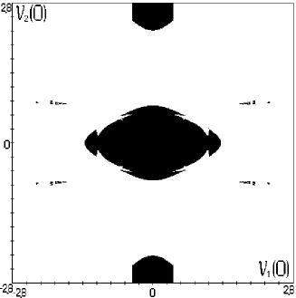
Figure 23: Stability diagram for the bush B$[a^{6},ai]$ in the FPU-$\beta$ chain.

References

- [1] G.M. Chechin, N.V. Novikova, A.A. Abramenko, Physica D 166 (2002) 208.
- [2] V.P. Sakhnenko, G.M. Chechin, Dokl. Akad. Nauk 330 (1993) 308 [Phys. Dokl. 38 (1993) 219];
- [3] V.P. Sakhnenko, G.M. Chechin, Dokl. Akad. Nauk 338 (1994) 42 [Phys. Dokl. 39 (1994) 625].
- [4] G.M. Chechin, V.P. Sakhnenko, Physica D 117 (1998) 43.
- [5] R.M. Rosenberg, J. Appl. Mech. 29 (1962) 7.
- [6] G.M. Chechin, A.V. Gnezdilov, M.Yu. Zekhtser, Int. J. Non-Linear Mech. 38 (2003) 1451.
- [7] G.M. Chechin, T.I. Ivanova, V.P. Sakhnenko, Phys. Status Solidi (b) 152 (1989) 431.
- [8] G.M. Chechin, E.A. Ipatova, V.P. Sakhnenko, Acta Cryst. A49 (1993) 824.
- [9] G.M. Chechin, V.P. Sakhnenko, H.T. Stokes, A.D. Smith, D.M. Hatch, Int. J. Non-Linear Mech. 35 (2000) 497.
- [10] G.M. Chechin, V.P. Sakhnenko, M.Yu. Zekhtser, H.T. Stokes, S. Carter, D.M. Hatch, in World Wide Web Proceedings of the Third ENOC Conference, http://www.midit.dtu.dk.
- [11] G.M. Chechin, O.A. Lavrova, V.P. Sakhnenko, H.T. Stokes, D.M. Hatch, Fizika tverdogo tela 44 (2002) 554.
- [12] G.M. Chechin, Comput. Math. Applic. 17 (1989) 255.
- [13] H.T. Stokes, D.M. Hatch, The software package ISOTROPY (this package is available on the Internet at http://www.physics.byu.edu/~stokesh/isotropy.html).
- [14] P. Poggi, S. Ruffo, Physica D 103 (1997) 251.
- [15] B. Rink, Physica D 175 (2003) 31.
- [16] S. Shinohara, J. Phys. Soc. Japan 71 (2002) 1802; S. Shinohara, Progr. Theor. Phys. Suppl. 150 (2003) 423.
- [17] G.M. Chechin, D.S. Ryabov, K.G. Zhukov, Construction of bushes of modes for the nonlinear monoatomic chains, Electronic journal “Investigated in Russia”, 137 (2003) 1616-1644, http://zhurnal.ape.relarn.ru/articles/2003/137.pdf.
- [18] K.V. Sandusky, J.B. Page, Phys. Rev. B 50 (1994) 866.
- [19] V.V. Krivtsova, G.M. Chechin, Crystallography 35 (1990) 1319.
- [20] G.M. Chechin, D.S. Ryabov, K.G. Zhukov, Investigation the stability of one-dimensional and two-dimensional bushes of vibrational modes for the Fermi-Pasta-Ulam chains, Electronic journal “Investigated in Russia”, 161 (2003) 1945-1964, http://zhurnal.ape.relarn.ru/articles/2003/161.pdf.