Analysis of Sunspot Number Fluctuations

Abstract

Monthly averages of the sunspot number visible on the sun, observed from 1749, Zurich Observatory, and from 1848 other observatories, have been analyzed. This time signal presents a frequency power spectra with a clear $1/f^{\alpha}$ behavior with $\alpha\simeq 0.8\pm 0.2$. The well known cycle of approximately 11 years, clearly present in the spectrum, does not produce a sensible distortion of that behavior. The eventual characterization of the sunspot time series as a fractal is analyzed by means of the detrended fluctuation analysis. The jump size distribution of the signal is also studied.

1 Introduction

A sunspot [1] is a relatively cool area on the solar face that appears as a dark blemish. The number of sunspots is continuously changing in time in a random fashion and constitutes a typical, a priori, random time series. Because of the symmetry of the twisted magnetic lines that originate sunspots, they are generally seen in pairs or in groups of pairs at both sides of the solar equator. As the sunspot cycle progresses, spots appear closer to the sun’s equator giving rise to the so called “butterfly diagram” in the latitude distribution. Magnetic fields about the sunspots are very strong and keep heat out of these regions on the sun surface. They are formed when magnetic field lines are twisted and poke through the solar photosphere. The twisted magnetic fields above sunspots are sites where solar flares are observed. It has been found that chromospheric flares show a very close statistical relationship with sunspots. This is illustrated by the Waldmeir relationship [1] between the mean number of flares per day, $E$, and the sunspot number, $R$, namely $E=0.061\,R$. Being the number of sunspots much larger than the corresponding to flares, it seems more appropriate for statistical analysis. Moreover, this connection between sunspots and solar magnetic field is particularly motivating for a further analysis of their frequency of appearance. In summary, being a consequence of the solar cycle, the variation of the number of sunspots is closely related to the so-called solar activity. In fact, the solar maximum activity corresponds to many sunspots present, while the minimum of activity is related to very few sunspots.

Another effect of the solar activity is the presence of fluctuations in the interplanetary magnetic field. Experimental data suggest [2] a $1/f$ dependence for the frequency spectra of its fluctuations in the range of large times, namely, $2.7\times 10^{-6}$ Hz to $1.8\times 10^{-5}$ Hz. In this analysis it is argued that on the basis of the observed behavior there is a superposition of signals with scale invariant distributions of correlation times. In other words, a kinematical superposition of signals due to scale-invariant reconnection of magnetic structures, near the solar surface, gives rise to the $1/f$ spectrum. It should be also noticed that at higher frequencies the interplanetary spectrum is known to have approximatively an $1/f^{5/3}$ behavior; this time associated with magnetohydrodynamics (MHD) homogeneous turbulence.

The result of our analysis of the sunspot number distribution along almost 250 years shows a clear correlation among all these phenomena.

After introducing the data and the different methods of analysis used, we present the results with a further comment on their implications.

2 Sunspot Data

There is experimental evidence and data registers on sunspots since Galileo (1610). Afterwards, the sunspot data were provided by the Zürich Observatory from 1749 to 1981. Since January 1981, the data are provided by the Sunspot Index Data Center (SIDC) [3].

In Figure 1 the monthly measured number of sunspots is plotted versus time. This plot includes $44,444$ data points. The approximate 11 years cycle can clearly be seen from this plot.

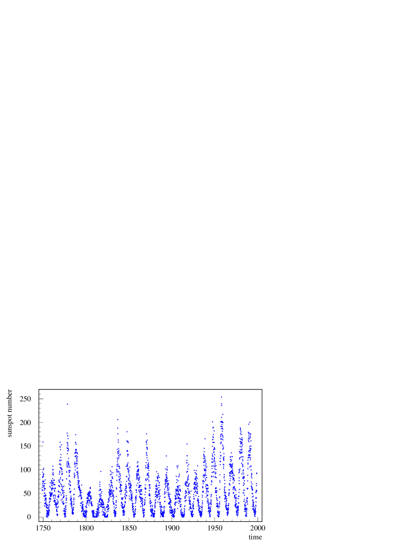
Figure 1: Observed spots number as a function of time

3 Analysis of the Time Series

The analysis of a given temporal signal with apparently random fluctuations starts by asking if the value of the signal in a given instant has any correlation with the signal in a later time. The standard statistical tool for describing the signal is the temporal correlation function and the corresponding power spectrum or frequency spectrum also called spectral density. In general, random time dependent perturbations give rise to random noise characterized by a frequency spectrum following a power law $1/f^{\beta}$ with $-2\leq\beta\leq 0$. Such a power law is found in a rich variety of physical systems exhibiting some kind of episodic activity. When $\beta\rightarrow 1$, the correlation times grow strongly. This behavior is closely related to the concept of fractal and self-similarity. In many cases, the dynamics of the corresponding physical system is attracted towards a critical state and the system is said to present self-organized criticality.

The concepts of fractal and self-similarity are directly related [4]. Fractals are self-similar under an isotropic reduction or scale transformation.

In many cases of interest, the concept of self-affine fractality or self-affinity has shown to be very fruitful. In this ”weak” form of similarity, the sequence of data looks alike when the reduction of the time scale is made with a different scaling factor than the one used for the measured variable. This means invariance under anisotropic scale changes. The random walk or Brownian movement defined by a function $B(t)$ that determines the instant position of the particle is a well-known example. If $B(0)=0$, then at any time $t$ the characteristic function of the random walk verifies $|\mu|^{-H_{1}}\,B(\mu\,t)$ for any $\mu\neq 0$. The Brownian exponent is precisely $H_{1}=1/2$. In any case it is possible to characterize the fractal behavior of a system through a non-integer dimension usually called fractal dimension $D$, related to the above mentioned $H_{1}$.

An alternative characterization of fractal time series is by means of the roughness or Hurst exponent $H_{u}=1+H_{1}$ that measures the persistency of the fluctuations related to the time series [5].

There have been different proposals for measuring these exponents. One of them is the analysis of the variance of increments at a given lag, also known with the geophysical name of semivariogram [6]. The detrended fluctuation analysis DFA [8] has shown to be an alternative procedure, some times a better one, for analyzing fluctuations in time series and a way of defining another similar exponent $H_{a}$. There are other possibilities as the mobile average analysis introduced in reference [9].

The statistical properties of the sunspot number fluctuations, were analyzed by means of the different tools just mentioned, plus the jump size distribution.

3.1 Analysis of the Frequency Power Spectrum

The analysis of correlation in time series starts with the temporal correlation function defined by

$$G(\tau)=\langle x(t_{0})\,x(t_{0}+\tau)\rangle_{t_{0}}-\langle x(t_{0})\rangle^{2}_{t_{0}}$$ (1)

Clearly, whenever no temporal correlation is present, one has $G(\tau)=0$. On the other hand, the rate with which $G(\tau)$ decreases from the average value of the instantaneous fluctuation towards zero measures the correlation time that evaluates the memory effects present in the signal.

The frequency spectrum is defined in terms of the amplitude of the Fourier transform of the time signal squared, namely

$$S(f)=\lim_{T\rightarrow\infty}\frac{1}{T}\,\left|\int^{T}_{-T}d\tau\,x(t)\,e^{2\,i\,\pi\,f\,\tau}\right|^{2}$$ (2)

In the particular case of a stationary process, i.e. its behavior is independent of the particular instant chosen to start the observation, the last expression ends in the cosine Fourier transform

$$S(f)=2\,\int_{0}^{\infty}d\tau\,G(\tau)\,\cos(2\pi f\tau)$$ (3)

In general, a random time dependent fluctuation gives rise to a random noise characterized by a frequency spectrum following a power law

$$S(f)\propto\frac{1}{f^{\beta}}$$ (4)

over a large range of frequencies, with well known examples in the range $-2\leq\beta\leq 0$.

There exists a heuristic argument showing the particular nature of the $\beta=1$ fluctuations that defines the so called $1/f$ noise. If $S(f)\propto 1/f^{\beta}$ and $G(\tau)\propto 1/\tau^{\gamma}$, then the cosine Fourier transform above roughly shows that $1/f^{\beta}$ has to be proportional to $1/f^{1-\gamma}$. Consequently, when $\beta$ approaches one, $\gamma$ has to vanish. This means that for $\beta=1$, the assumed form of $G(\tau)$ is replaced by a logarithmic behavior implying a much lower rate of decreasing of the correlation i.e. correlation times grow strongly.

Another case of particular interest is the exponent $\beta=5/3$ corresponding to the homogeneous turbulence in fluids. The analogy is related to the presence of hierarchical processes like cascades from large to small scale fluctuations.

The analysis of sunspot data along the lines just described provided an exponent clearly compatible with $\beta=1$ as it is shown in figure 2.

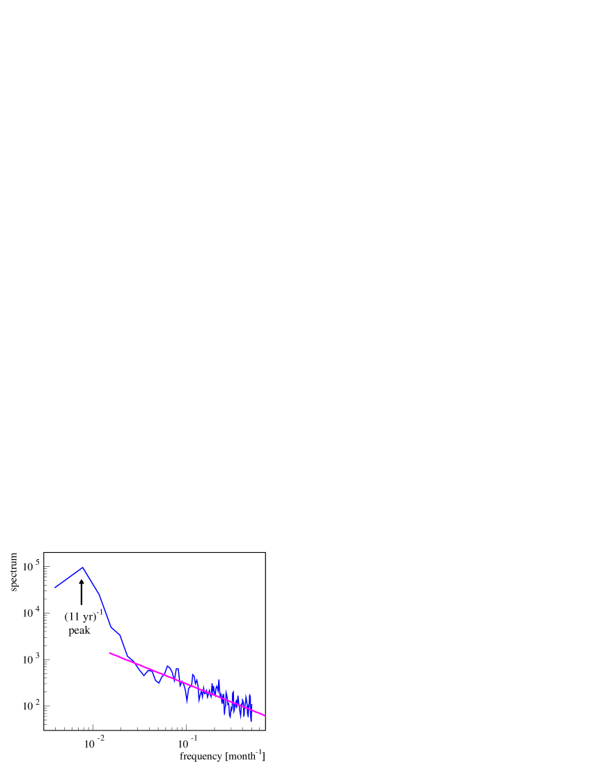
Figure 2: Power spectrum of the sunspot number fluctuation. The arrow indicates the peak at $f=(11\;{\rm yr})^{-1}=0.0076\;{\rm month}^{-1}$.

In order to improve the analysis, a standard Butterworth filter [7] ( $1/[1+\omega^{2\,n}]$ ) for $n=6$ and $8$, was applied to the data in order to separate the evident low frequency components of the signal under consideration from the high frequency ones. The low frequency part shows clearly the well known $\sim 11$ year period of activity as a sharp peak in the corresponding spectrum, while the high frequency component has the noisy behavior presented in figure 2. A power spectrum study of this high frequency part provides the result

$$P(f)\approx f^{-0.8\pm 0.2}$$

for

$$1/(132\,\mathrm{month})<f<(1/1\,\mathrm{month})$$

or alternatively

$$1.3\,\times\,10^{-10}\,\mathrm{Hz}<f<4\,\times\,10^{-7}\,\mathrm{Hz}$$

We then conclude that the power spectrum of the sunspot number temporal fluctuations, along more than two hundred years, is well represented by a $1/f$ behavior.

3.2 Detrended Fluctuation Analysis (DFA)

DFA [8] is an alternative statistical method to classify temporal correlations in a time series. It consists in dividing the time series of $n$ values $x(t)$ into $n/s$ nonoverlapping groups, each with $s$ values. Inside each group, the local trend or tendency $y(t)=a\,t+b$ is defined as usual through the linear least-square fit of the values in the group. From this, the detrended fluctuation function $F(s)$ is defined as

$$\left[F(s)\right]^{2}=\frac{1}{s}\,\sum^{(k+1)s}_{t=ks+1}\,\left[x(t)-y(t)\right]^{2}\,\,\,\,;\,\,\,\,k=0,1,\ldots,\left(\frac{n}{s}-1\right)$$ (5)

Finally, the average of $F(s)$ over the $n/s$ intervals is computed.

Whenever the time series data $x(t)$ is randomly uncorrelated (or short range correlated), the expected behavior for the average is a power law, namely

$$\langle F(s)\rangle\sim s^{H_{a}}$$ (6)

with an exponent $H_{a}=1/2$, characteristic value of a random walk. If for a given range of $s$ the exponent $H_{a}$ happens to be different from $1/2$, it detects the presence of long-range correlations in that range. When $H_{a}>1/2$ there is a persistent behavior or a positive correlation between the increments, while if $H_{a}<1/2$ the behavior is antipersistent showing the presence of a negative correlation. In both cases it is customary to speak, after Mandelbrot, about fractional Brownian movement.

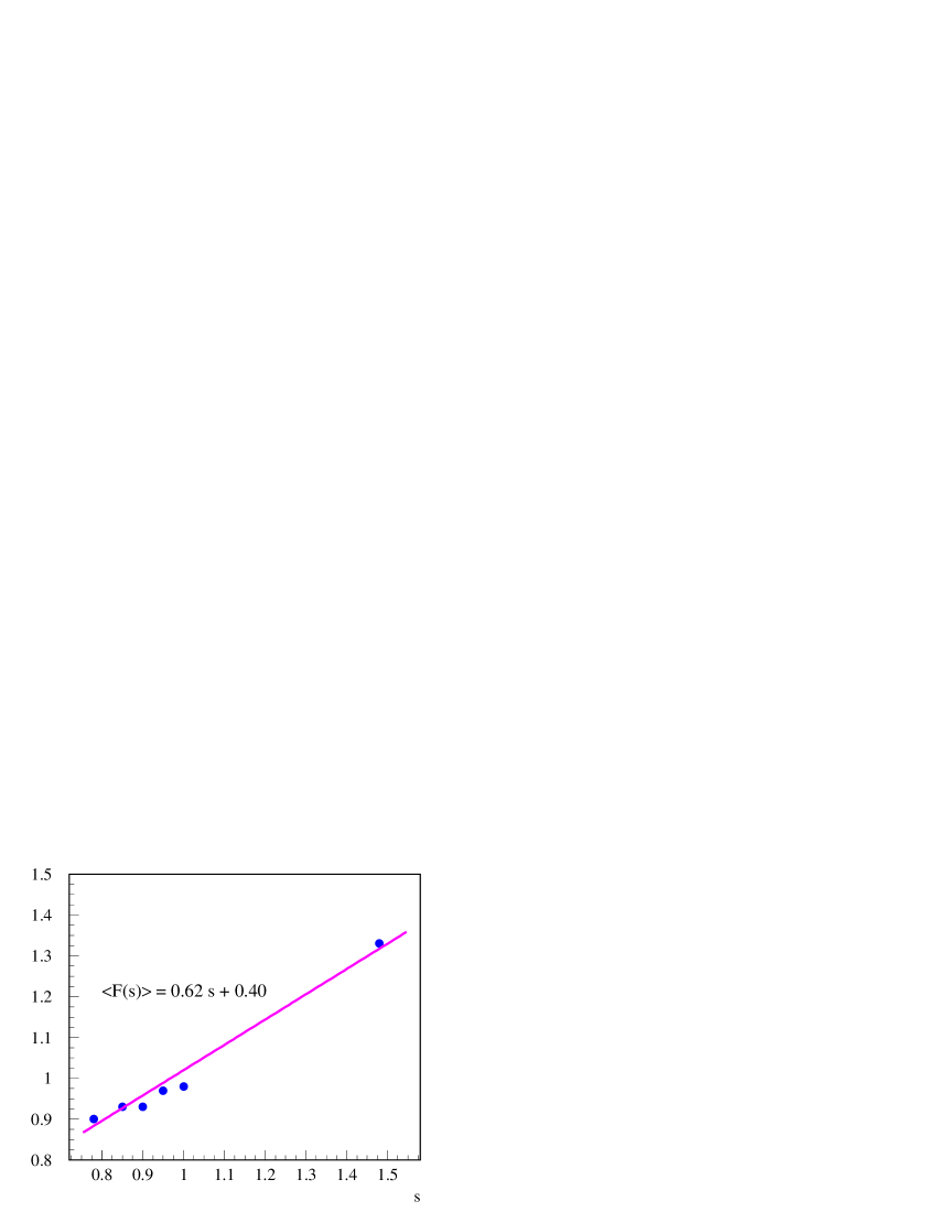
Figure 3: Average of the detrended fluctuation.

The DFA avoids inherent trends at all scales and allows to easily probe local correlations. Notice also that $H_{a}$ is related to the fractal dimension through

$$D=2-H_{a}$$ (7)

if the distribution is described in a two dimensional space as is the case for the time series under analysis.

The behavior of the detrended fluctuation function for sunspot data is shown in figure 3. We found the presence of a persistent behavior characterized by the exponent $H_{a}=0.62$.

3.3 Jump-Size Distribution Method

A further analysis of the time series can be performed in terms of the jump-size distribution. The main objective is to determine the probability distribution of the logarithm of consecutive relative jumps in the number $S_{i}$ of sunspots, namely

$$L_{i}=\log\left|\frac{S_{i}}{S_{i+1}}-1\right|$$ (8)

together with the corresponding distribution

$$F_{L}=Prob(\overline{L}\leq L)$$ (9)

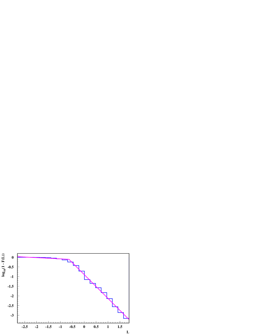
Figure 4: Logarithm of the cumulative distribution of consecutive relative jumps, $\log_{10}[1-F_{L}(L)]$ (see equation (9)), plotted versus $L$ for the case of the number of sunspots

In figure 4, $\log_{10}[1-F_{L}(L)]$ is displayed for the case of the sunspot number using the data plotted in figure 1. It is found that $F_{L}$ shows an inverse power behavior of the Zipf type [10], i.e., a straight line on a double logarithmic plot, showing that $[1-F_{L}(L)]$ can be expressed as the power

$$1-F_{L}(L)=L^{-\tau}$$ (10)

We have found two different regimes: The one corresponding to negative $L$ with $\tau_{1}\approx 0$, and the one corresponding to positive $L$, characterized by

$$\tau_{2}=1.23\pm 0.20.$$ (11)

In the Appendix we have included an analysis of the probability distribution of relative increments, just to explicitly show that this power behavior should be expected particularly in the case of a probability distribution of events following a power law.

4 Final Comments

It is well-known that the $1/f$ noise is one of the most common and ubiquitous features in Nature. Superposition of effects giving rise to signals with scale invariant distributions of correlation times, the so-called scale similarity, could be on the basis of the observed behavior. However, a proper explanation for such a behavior is still lacking and for that reason, the physical origin of the $1/f$ noise is pretty much an open question. Nevertheless, a recent analysis [11] of models presenting self-organized criticality seems to indicate that the origin of the $1/f$ behavior could be found in the superposition of local power-spectra with characteristic frequencies suitably distributed in space and having spectra that do not present the $1/f$ behavior. It has been also shown, in the mentioned context, that one of the main features relevant for describing $1/f$ noise is the well-known process of activation/deactivation.

We find that both mentioned ingredients are present in the case of sunspots. In fact, the noise in the magnetic field measured at earth, for short times (large frequencies) even during magnetic storms, presents a $1/f^{2}$ spectrum. Consequently, the property of the sunspots spectrum can be related to the interference of random distributed magnetic disturbances. Moreover, the commonly accepted mechanism for the sunspot appearance is an activation/deactivation process, as it was discussed in the introduction.

With reference to the roughness exponent, one can conclude that it also detects the persistent behavior or positive correlation between increments, due to the physical mechanisms giving rise to sunspots.

Appendix: On Probability Distribution of Relative Increments

In this Appendix we illustrate how the uniform and the power distributions give rise to the probability distribution of relative increments of the Zipf-like type. To start with, let us consider a random variable $X$ with probability distribution $f_{X}(x)$ ($-\infty<x<\infty$). The distribution $f_{X}$ is normalized, that is,

$$\int_{-\infty}^{\infty}f_{X}(x)dx=1.$$ (A.1)

The cumulative probability distribution $F_{X}(x)$ is defined via:

$$F_{X}(x)=\int_{-\infty}^{x}f_{X}(z)dz.$$ (A.2)

$F_{X}(x)$ gives the probability that $X\leq x$, and clearly, $f_{X}(x)=dF_{X}(x)/dx$. Let $x_{i}$, $i=1,2,\ldots$, be a series of independent instances of $X$, that is, each $x_{i}$ is an independent sample of the distribution $f_{X}(x)$. We are interested in calculating the probability distribution of certain functions of these numbers, namely, $r_{i}$, $R_{i}$ and $L_{i}$, $i=1,2,\ldots$ defined as

$$\displaystyle r_{i} = \displaystyle{{x_{i}}\over{x_{i+1}}}-1$$ (A.3)

$$R_{i} = |r_{i}|$$ (A.4)

$$L_{i} = \ln R_{i}$$ (A.5)

The probability distribution of the $r_{i}$’s can be evaluated as follows (overlined symbols refer to random variables):

$$F_{r}(r) = \hbox{Prob}(\overline{r}\leq r)$$ (A.6)

$$= \displaystyle\hbox{Prob}\!\left({{x_{i}}\over{x_{i+1}}}-1\leq r\right)$$ (A.7)

$$= \displaystyle\hbox{Prob}(x_{i}\leq(r+1)x_{i+1}).$$ (A.8)

Since $x_{i}$ and $x_{i+1}$ are independent, the probability of the last equation can be evaluated straightforwardly

$$F_{r}(r)=\hbox{Prob}(x_{i}\leq(r+1)x_{i+1})=\int_{-\infty}^{\infty}f_{X}(x_{i+1})F_{X}\left((r+1)x_{i+1}\right)\,dx_{i+1}.$$ (A.9)

Or, equivalently,

$$F_{r}(r)=\int_{-\infty}^{\infty}dx_{1}f_{X}(x_{1})\int_{-\infty}^{(r+1)x_{1}}dx_{2}f_{X}(x_{2}).$$ (A.10)

The probability density distribution, $f_{r}$, can be then evaluated via:

$$f_{r}(r)={{dF_{r}(r)}\over{dr}}=\int_{-\infty}^{\infty}dx\>x\,f_{X}(x)\,f_{X}((r+1)x).$$ (A.11)

The distributions for $R$ and $L$ can be calculated similarly:

$$F_{R}(R)=\hbox{Prob}(\overline{R}\leq R)=\hbox{Prob}(|r|\leq R).$$ (A.12)

It is evident that $F_{R}(R)=0$ for $R\leq 0$. For $R>0$ one has,

$$F_{R}(R)=\hbox{Prob}(-R\leq r\leq R)=F_{r}(R)-F_{r}(-R).$$ (A.13)

On the other hand,

$$F_{L}(L) = \hbox{Prob}(\overline{L}\leq L)$$ (A.14)

$$= \hbox{Prob}(\ln R\leq L)$$ (A.15)

$$= \hbox{Prob}(R\leq e^{L}),$$ (A.16)

therefore,

$$F_{L}(L)=F_{R}(e^{L}).$$ (A.17)

The probability density distribution can be then calculated similarly as in equation (A.11).

Let us now evaluate these probability distributions for the particular cases of the uniform and the power distributions.

The uniform distribution

The uniform distribution is given by

$$f_{X}(x)=\left\{\begin{array}[]{ll}1&\hbox{if\ }0\leq x\leq 1\\[16.0pt] 0&\hbox{otherwise}\end{array}\right.$$ (A.18)

Applying equation (A.10), one obtains

$$F_{r}(r)=\left\{\begin{array}[]{ll}0&\hbox{if\ }r<-1\\[16.0pt] \displaystyle{{r+1}\over{2}}&\hbox{if\ }-1\leq r\leq 0\\[16.0pt] \displaystyle{{2r+1}\over{2(r+1)}}&\hbox{if\ }r>0\end{array}\right.$$ (A.19)

And then from equation (A.13)

$$F_{R}(R)=\left\{\begin{array}[]{ll}0&\hbox{if\ }R\leq 0\\[16.0pt] \displaystyle{{2R+1}\over{2(R+1)}}-{{1-R}\over{2}}&\hbox{if\ }0<R<1\\[16.0pt] \displaystyle{{2R+1}\over{2(R+1)}}&\hbox{if\ }R\geq 1\end{array}\right.$$ (A.20)

The power distribution

Consider the distribution

$$f_{X}(x)=\left\{\begin{array}[]{ll}(\alpha-1)x^{-\alpha}&\hbox{if\ }x>1\\[16.0pt] 0&\hbox{otherwise}\end{array}\right.$$ (A.21)

where $\alpha$ is a real parameter ($\alpha>1$).

Applying equation (A.10), one obtains

$$F_{r}(r)=\left\{\begin{array}[]{ll}0&\hbox{if\ }r<-1\\[16.0pt] \displaystyle(r+1)^{\alpha}\left({1\over{r+1}}-{1\over 2}\right)&\hbox{if\ }-1<r<0\\[16.0pt] \displaystyle 1-{1\over{2(r+1)^{\alpha-1}}}&\hbox{if\ }r>0\end{array}\right.$$ (A.22)

And then from equation (A.13)

$$F_{R}(R)=\left\{\begin{array}[]{ll}0&\hbox{if\ }R\leq 0\\[16.0pt] \displaystyle 1-{1\over{2(R+1)^{\alpha-1}}}-(1-R)^{\alpha}\left({1\over{1-R}}-{1\over{2}}\right)&\hbox{if\ }0<R<1\\[16.0pt] \displaystyle 1-{1\over{2(R+1)^{\alpha-1}}}&\hbox{if\ }R\geq 1\end{array}\right.$$ (A.23)

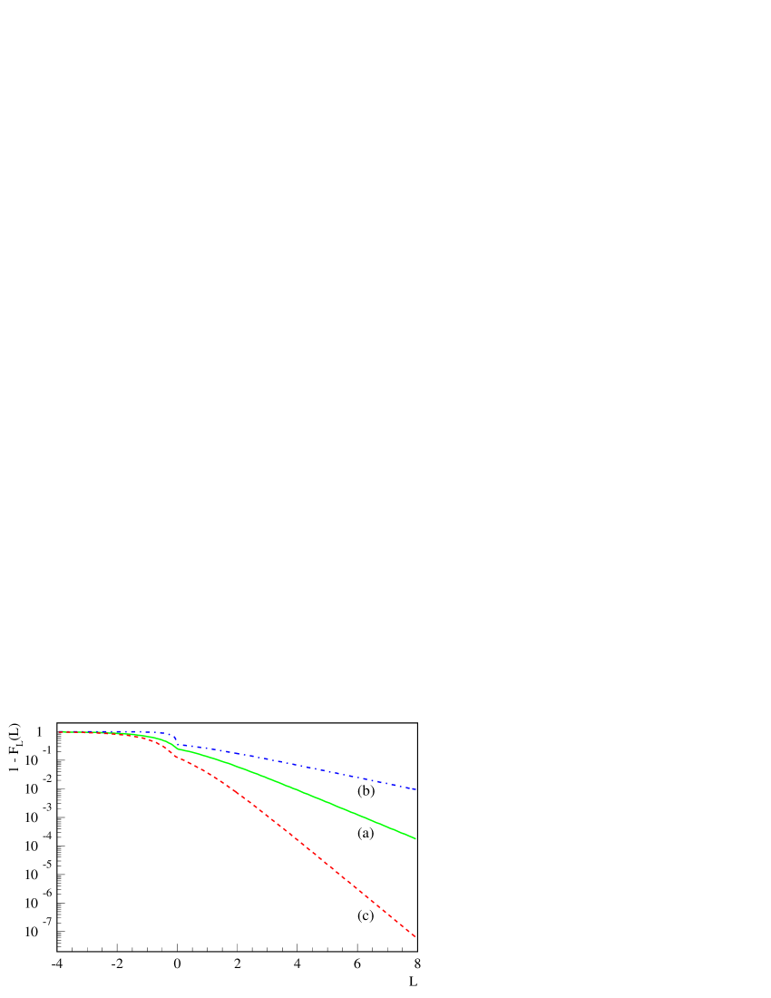
Figure 5: Some cumulative functions ($1-F_{L}(L)$) plotted versus $L$. (a) The uniform distribution (equation (A.20)). (b) The power distribution (equation (A.23)) in the case $\alpha=3/2$. (c) Same as (b) but for $\alpha=3$. In every case two asymptotic regimes are clearly seen.

In these two examples, two different straight line regimes are clearly present, as it is illustrated in figure 5 where $1-F_{L}(L)$ (see equation (A.17)) is plotted as a function of $L$. This is precisely the behaviour of the corresponding distribution in the case of the sunspot number, as shown in section 3.3 (figure 4).

References

- [1] see for example Sunspots by R.J. Bray, R.E. Loughhead, Dover Publications, New York 1979.
- [2] W.H. Matthaeus, M.L. Goldstein, Phys. Rev. Lett., 57, 495 (1986).
- [3] http://www.oma.be/KSB-ORB/SIDC/index.html
- [4] B.B. Mandelbrot, The Fractal Geometry of Nature, Freeman, N.York (1982).
- [5] E.A. Peters, Chaos and Order in the Capital Markets, J. Wiley (1991).
- [6] P.A. Burrough, Nature, 294, 240 (1981).
- [7] A. Zverev, Handbook of Filter Synthesis, John Wiley (1967).
- [8] C.K. Peng et al., Phys. Rev. E, 49, 1685 (1994).
- [9] N. Vandewalle, M. Ausloos, Phys. Rev. E, 58, 6832 (1999).
- [10] see for example “How Nature Works” by P. Bak, Oxford University Press, 1997.
- [11] P. De Los Rios, Yi-Cheng Zhang, Phys. Rev. Lett., 82, 472 (1999).
- [12] P. Bak, C. Tang, K. Wiesenfeld, Phys. Rev. Lett., 59, 381 (1987).
- [13] M. B. Weissman, Rev. Mod. Phys., 60, 537 (1988).
- [14] S. L. Miller, W. M. Miller, P. J. McWhorter, J. Appl. Phys., 73, 2617 (1993).