Intermediate statistics in quantum maps

Abstract

We present a one-parameter family of quantum maps whose spectral statistics are of the same intermediate type as observed in polygonal quantum billiards. Our central result is the evaluation of the spectral two-point correlation form factor at small argument, which in turn yields the asymptotic level compressibility for macroscopic correlation lengths.

1 Introduction

The classification of quantum systems according to universal statistical properties is one of the central objectives in the study of quantum chaos. It is generally believed that the spectral statistics of systems with chaotic classical limit are governed by random matrix ensembles, while systems with integrable classical dynamics follow the statistical properties of independent random variables from a Poisson process [1, 2, 3]. Interestingly, certain billiards in rational polygons fall in neither of the two universality classes: the energy level correlations are conjectured to be of intermediate type [4, 5, 6, 7, 8]. In particular, this means that the consecutive level spacing distribution $P(s)$ exhibits level repulsion similar to random matrix eigenvalues, but has an exponential tail as for independent random variables. Furthermore, the spectral form factor $K_{2}(\tau)$ is intermediate between 0 and 1 in the limit $\tau\to 0$. One standard example for a statistics of this type is the semi-Poisson distribution, for which $P(s)=4s\exp(-2s)$ and $K_{2}(\tau\to 0)=1/2$.

Figure 1: The consecutive level spacing distribution for Hilbert space dimension $N=7001$ and $\alpha=1/2$ (left) and $\alpha=2/3$ (right). The Poisson distribution corresponds to $P(s)=\exp(-s)$, semi-Poisson to $P(s)=4s\exp(-2s)$, and COE to the level spacing distributions of the circular orthogonal random matrix ensembles.

Figure 2: The consecutive level spacing distribution for Hilbert space dimension $N=7001$ and $\alpha=3/5$ (left) and $\alpha=5/8$ (right).

Figure 3: The consecutive level spacing distribution for $\alpha=(\sqrt{5}-1)/2$ and Hilbert space dimensions $N=6997$ (left) and $N=5867$ (right) corresponding to values of $\epsilon\sqrt{N}\simeq 32.1$ and $\epsilon\sqrt{N}=0.41$, respectively.

In this paper we present a one-parameter family of quantum maps whose spectral statistics are of a similar intermediate type as observed in polygonal billiards, cf. Figs. 1 and 2. The main result of our investigation is the evaluation of the spectral form factor $K_{2}(\tau)$ at small argument. It is based on a number-theoretic analysis which turns out to be considerably easier than the geometric approach required for billiards [7].

Consider the following map of the two-torus ${\mathbb{T}}^{2}={\mathbb{R}}^{2}/{\mathbb{Z}}^{2}$,

$$\Phi_{f}:{\mathbb{T}}^{2}\to{\mathbb{T}}^{2},\quad\begin{pmatrix}p\\ q\end{pmatrix}\mapsto\begin{pmatrix}p+f(q)\\ q+2(p+f(q))\end{pmatrix}$$ (1)

where $f$ is some $1$-periodic function. The map is a concatenation $\Phi_{f}=\Phi_{0}\circ\rho_{f}$ of free motion $\Phi_{0}$ and kick $\rho_{f}$,

$$\Phi_{0}:\begin{pmatrix}p\\ q\end{pmatrix}\mapsto\begin{pmatrix}p\\ q+2p\end{pmatrix},\quad\rho_{f}:\begin{pmatrix}p\\ q\end{pmatrix}\mapsto\begin{pmatrix}p+f(q)\\ q\end{pmatrix}.$$ (2)

The quantization of a torus map associates with it a unitary operator acting on the $N$-dimensional Hilbert space of functions $\psi:{\mathbb{Z}}_{N}\to{\mathbb{C}}$ with inner product $\langle\psi|\phi\rangle=N^{-1}\sum_{Q=0}^{N-1}\psi^{*}(Q)\phi(Q)$. Here ${\mathbb{Z}}_{N}={\mathbb{Z}}/N{\mathbb{Z}}$ denotes the integers modulo $N$, and $N$ has the physical interpretation of an inverse Planck’s constant. The quantum evolution operators $U(\Phi_{0})$ and $U(\rho_{f})$ corresponding to $\Phi_{0}$ and $\rho_{f}$, respectively, are defined by the matrix elements (cf. [9, 10, 11, 12])

$$\langle Q^{\prime}|U(\Phi_{0})|Q\rangle=\frac{1}{N}\sum_{P=0}^{N-1}e_{N}\left(-P^{2}+P(Q^{\prime}-Q)\right),$$ (3)

$$\langle Q^{\prime}|U(\rho_{f})|Q\rangle=\langle Q^{\prime}|Q\rangle\;e\left(-NV\left(\tfrac{Q}{N}\right)\right),$$ (4)

where $V(q)$ is a periodic function defined by $f(q)=-V^{\prime}(q)$, and $e_{N}(x)=\exp(2\pi\textrm{i}x/N)$ and $e(x)=\exp(2\pi\textrm{i}x)$. Furthermore $U(\Phi_{f})=U(\Phi_{0})U(\rho_{f})$ and thus

$$\langle Q^{\prime}|U(\Phi_{f})|Q\rangle=\langle Q^{\prime}|U(\Phi_{0})|Q\rangle\;e\left(-NV\left(\tfrac{Q}{N}\right)\right).$$ (5)

We are interested in the special case of the piecewise linear sawtooth potential $V(q)=-\alpha\{q\}$ for some real constant $\alpha$, where $\{q\}$ denotes the fractional part of $q$. In this case $f(q)=\alpha$. The corresponding classical map $\Phi_{\alpha}:=\Phi_{f}$ is uniquely ergodic for irrational $\alpha$ (in particular, there are no periodic orbits) but not mixing. For rational $\alpha$, the motion can be identified with an interval-exchange transformation. Note that in the momentum representation $|P\rangle$, with $\langle Q|P\rangle=N^{-1/2}e_{N}(PQ)$, the operator $U(\Phi_{\alpha})$ has the representation

$$\langle P^{\prime}|U(\Phi_{\alpha})|P\rangle=\frac{1}{N}\,e_{N}(-{P^{\prime}}^{2})\,\frac{1-e(N\alpha)}{1-e_{N}(P-P^{\prime}+N\alpha)}$$ (6)

if $N\alpha\notin{\mathbb{Z}}$ and

$$\langle P^{\prime}|U(\Phi_{\alpha})|P\rangle=e_{N}(-{P^{\prime}}^{2})\langle P^{\prime}|P+N\alpha\rangle$$ (7)

otherwise.

Since $U(\Phi_{\alpha})$ is unitary its eigenvalues are of the form $\exp(\textrm{i}\theta_{j})$ with eigenphases $0\leq\theta_{1}\leq\theta_{2}\leq\cdots\leq\theta_{N}<2\pi$; it is convenient to set $\theta_{0}:=\theta_{N}-2\pi$. The spacing distribution for consecutive levels is described by the probability density

$$P(s)=\frac{1}{N}\sum_{j=1}^{N}\delta\left(s-\frac{N}{2\pi}(\theta_{j}-\theta_{j-1})\right),$$ (8)

where the factor of $N/2\pi$ ensures that $s$ measures spacings on the scale of the mean level spacing $2\pi/N$. Figs. 1-3 display the spacing distribution $P(s)$ of the eigenphases of the matrix $U(\Phi_{\alpha})$ for both rational (Figs. 1-2) and irrational (Fig. 3) values of $\alpha$, and $N$ a prime number. In the case of rational $\alpha=a/b$ one should avoid Hilbert space dimensions $N$ divisible by $b$, since the matrix (7) has highly singular statistics [18, 19]. For irrational $\alpha$, we find in Fig. 3 (left) a spacing distribution which resembles those of random matrices from the the Circular Orthogonal Ensemble (COE). COE statistics are normally expected for systems with chaotic classical limit and time-reversal symmetry [2, 3]. In our case the time-reversal transformation which anti-commutes with $U(\Phi_{\alpha})$ is $T^{\prime}=U(\Phi_{0})^{1/2}\,T\,U(\Phi_{0})^{-1/2}$, where $T$ denotes the complex conjugation operator $T\psi:=\psi^{*}$. Localized spacing distributions of the type seen in Fig. 3 (right) occur when $\epsilon$, defined as the oriented distance of $N\alpha$ to the nearest integer, is of the order $1/\sqrt{N}$. Such correlations arise as the perturbation of a rigid spectrum, and will be described in section 3.

The map $\Phi_{\alpha}$ has in fact a further classical symmetry: it commutes with $\rho_{1/2}$ for any $\alpha$. Thus, for $N$ even, the corresponding operators $U(\Phi_{\alpha})$ and $U(\rho_{1/2})$ commute and the eigenstates of $U(\Phi_{\alpha})$ fall into two parity classes according to $U(\rho_{1/2})\varphi_{j}=\varphi_{j}$ or $U(\rho_{1/2})\varphi_{j}=-\varphi_{j}$, respectively. Our numerical experiments suggest that the level statistics for each subspectrum for even $N$ are of the same type as those for odd $N$ displayed in Figs. 1-3.

A statistics which is more accessible from an analytical point of view is the two-point correlation density (which describes the distribution of all spacings)

$$R_{2}(s)=\frac{1}{N}\sum_{j,k=1}^{N}\sum_{m\in{\mathbb{Z}}}\delta\left(s-\frac{N}{2\pi}(\theta_{j}-\theta_{k}+2\pi m)\right).$$ (9)

The Poisson summation formula applied to the $m$-sum yields

$$R_{2}(s)=\frac{1}{N^{2}}\sum_{n\in{\mathbb{Z}}}\big{|}\operatorname{Tr}\left[U(\Phi_{\alpha})^{n}\right]\big{|}^{2}e_{N}(ns).$$ (10)

The spectral form factor is defined as the Fourier transform of $R_{2}(s)$,

$$K_{2}(\tau)=\frac{1}{N}\big{|}\operatorname{Tr}\left[U(\Phi_{\alpha})^{n}\right]\big{|}^{2},\quad\tau=n/N.$$ (11)

In the following section we will calculate

$$\overline{K_{2}(0)}:=\lim_{n\to\infty}\lim_{N_{\nu}\to\infty}\frac{1}{n}\sum_{n^{\prime}=1}^{n}K_{2}(n^{\prime}/N)$$ (12)

where the limit is taken along suitable subsequences $N_{1},N_{2},\ldots\to\infty$ of integers. To illustrate the relevance of this quantity, let us consider the counting function ${\mathcal{N}}(L,\xi)$ for the number of eigenphases in the interval $[\xi-\frac{\pi L}{N},\xi+\frac{\pi L}{N}]$ (mod $2\pi$). The number variance is defined by

$$\Sigma^{2}(L) =\frac{1}{2\pi}\int_{0}^{2\pi}[{\mathcal{N}}(L,\xi)-L]^{2}d\xi$$ (13)

$$=\frac{L}{N}\sum_{j,k=1}^{N}\sum_{m\in{\mathbb{Z}}}\zeta\left(\frac{N}{2\pi L}(\theta_{j}-\theta_{k}+2\pi m)\right)-L^{2}$$ (14)

with $\zeta(x)=\int_{\mathbb{R}}\chi(x-y)\chi(y)dy=\max\{1-|x|,0\}$, where $\chi$ is the indicator function of the interval $[-\frac{1}{2},\frac{1}{2}]$. In view of (9), (10) and (14), number variance and form factor are related by

$$\Sigma^{2}(L)=\frac{L^{2}}{N^{2}}\sum_{n\neq 0}\big{|}\operatorname{Tr}\left[U(\Phi_{\alpha})^{n}\right]\big{|}^{2}\;\widehat{\chi}\left(\frac{L}{N}\,n\right)^{2}$$ (15)

where $\widehat{\chi}(y)=\sin(\pi y)/(\pi y)$ is the Fourier transform of $\chi$. It then follows from (12) and a standard probabilistic argument that, for macroscopic intervals of size $L=\ell N$ (with $\ell>0$ fixed as $N_{\nu}\to\infty$), we have

$$\lim_{\ell\to 0}\lim_{\begin{subarray}{c}N_{\nu}\to\infty\\ L=\ell N_{\nu}\end{subarray}}\frac{\Sigma^{2}(L)}{L}=\overline{K_{2}(0)}$$ (16)

since $\ell\sum_{k\neq 0}\widehat{\chi}(k\ell)^{2}\to\int\widehat{\chi}(y)^{2}dy=1$, as $\ell\to 0$. The ratio $\Sigma^{2}(L)/L$ is called the level compressibility [8].

2 Spectral form factor at small argument

To calculate the value of $K_{2}(\tau)$ at small but non-zero values of $\tau$, we note that in the semiclassical limit $N\to\infty$, the trace $\operatorname{Tr}U(\Phi_{\alpha})^{n}$ is asymptotically equal to $\operatorname{Tr}U(\Phi_{\alpha}^{n})$, with $n$ arbitrary but fixed. This may be seen by representing the respective traces as Gutzwiller-type periodic orbit sums.

The advantage of the choice of $\Phi_{\alpha}$ over other piecewise linear maps is that there is an explicit formula for the $n$th iterate. (We have observed intermediate statistics also for the closely related “triangle maps” introduced by Casati and Prosen [13]; the classical analysis of these maps is however considerably more involved.) Here, a short calculation shows that

$$\Phi_{\alpha}^{n}=\rho_{(n-1)\alpha/2}\circ\Phi_{0}^{n}\circ\rho_{(n+1)\alpha/2}.$$ (17)

The corresponding quantum evolution is therefore given by

$$\langle Q^{\prime}|U(\Phi_{\alpha}^{n})|Q\rangle=e\left(N\left(\tfrac{n-1}{2}\right)\alpha\left\{\tfrac{Q^{\prime}}{N}\right\}\right)\langle Q^{\prime}|U(\Phi_{0}^{n})|Q\rangle e\left(N\left(\tfrac{n+1}{2}\right)\alpha\left\{\tfrac{Q}{N}\right\}\right),$$ (18)

and so

$$\operatorname{Tr}U(\Phi_{\alpha}^{n})=\frac{1}{N}\sum_{P=0}^{N-1}e_{N}(-nP^{2})\times\sum_{Q=0}^{N-1}e(n\alpha Q)$$ (19)

where the first sum is a classical Gauss sum and the second a geometric sum. Let $m:=2n/\gcd(2n,N)$ and $M:=N/\gcd(2n,N)$, then

$$\left|\sum_{P=0}^{N-1}e_{N}(-nP^{2})\right|=\frac{N}{M}\left|\sum_{P=0}^{M-1}\exp\left(\pi\textrm{i}P^{2}\tfrac{m}{M}\right)\right|$$ (20)

which evaluates to $N/\sqrt{M}$ if $Mm$ is divisible by 2, and vanishes otherwise. The geometric sum is $O(1)$ for irrational $\alpha$ and $n\neq 0$ and hence $K_{2}(n/N)\sim 0$ for all bounded $n$ in this case. For rational $\alpha=a/b$, the geometric sum equals $N$ if $n$ is divisible by $b$ and is $O(1)$ otherwise. Thus $K_{2}(n/N)\sim\gcd(2n,N)$ provided $n$ is divisible by $b$ and $2Nn/\gcd(2n,N)^{2}$ is divisible by 2; $K_{2}(n/N)\sim 0$ in all other cases.

If we restrict ourselves to a subsequence of the values of $N$ which are prime numbers then $\gcd(2n,N)=1$ for $n<N$, and the time averaged form factor is

$$\overline{K_{2}(0)}:=\lim_{n\to\infty}\lim_{\begin{subarray}{c}N\to\infty\\ \text{$N$ prime}\end{subarray}}\frac{1}{n}\sum_{n^{\prime}=1}^{n}K_{2}(n^{\prime}/N)=\frac{1}{b}.$$ (21)

These values of $\overline{K_{2}(0)}$ are consistent with those expected for intermediate statistics [7]. The case $b=2$ and $N$ prime, for which $\overline{K_{2}(0)}=1/2$, does however not agree with the Poisson statistics seen numerically in Fig. 1 (left), where $\overline{K_{2}(0)}=1$. The solution to this apparent paradox is that $P(s)$ displays correlations on the scale of the mean level spacing, whereas $\overline{K_{2}(0)}$ involves correlations on much larger scales of order $N$. Similar discrepancies between a random matrix-like $P(s)$ and a non-universal $K_{2}(\tau\approx 0)$ have been observed for non-arithmetic Hecke triangles [14, 15], compact hyperbolic triangles and tetrahedra [16] and cat maps coupled to a spin $1/2$ [17].

If $N$ is twice a prime, i.e., $N=2R$ with $R$ an odd prime, then $\gcd(2n,N)=2$ for $n<R$, and $2Nn/4=Rn$ is divisible by 2 if and only if $n$ is even. Hence only terms with $n$ divisible by $\operatorname{lcm}(2,b)$ contribute, and so

$$\overline{K_{2}(0)}:=\lim_{n\to\infty}\lim_{\begin{subarray}{c}N\to\infty\\ \text{$N/2$ prime}\end{subarray}}\frac{1}{n}\sum_{n^{\prime}=1}^{n}K_{2}(n^{\prime}/N)=\frac{2}{\operatorname{lcm}(2,b)}.$$ (22)

The situation is different for $N=\rho R$, where $\rho$ is a fixed odd prime, and $R$ runs again over all odd primes. Now $\gcd(2n,N)=\gcd(n,\rho)$ for $n<R$, and $2Nn/\gcd(n,\rho)^{2}$ is always divisible by 2. Since $\rho$ is prime, $\gcd(n,\rho)=1$ if $n$ is not divisible by $\rho$ and $\gcd(n,\rho)=\rho$ if it is. In this case

$$\overline{K_{2}(0)}:=\lim_{n\to\infty}\lim_{\begin{subarray}{c}N\to\infty\\ \text{$N/\rho$ prime}\end{subarray}}\frac{1}{n}\sum_{n^{\prime}=1}^{n}K_{2}(n^{\prime}/N)=\frac{1}{b}+\frac{\rho-1}{\operatorname{lcm}(\rho,b)}.$$ (23)

Figure 4: Left: Level compressibility $\Sigma^{2}(L)/L$ with $L=100$ for rational $\alpha=a/b$ ($\times$), versus $\overline{K_{2}(0)}$ ($\odot$). From top to bottom: $N=7001$ (Equation (21)), $N=6998$ (Equation (22)), and $N=6999$ (Equation (23)). Right: numerical value of the form factor and theoretical plot (24) with $K_{2}(0)$ given by $\overline{K_{2}(0)}$, for the same $N$ and $\alpha=1/4$.

Fig. 4 (left) illustrates the asymptotic relation (16) between the level compressibility and $\overline{K_{2}(0)}$ for large values of $N$: a prime ($N=7001$), twice a prime ($N=6998$) and three times a prime ($N=6999$). Fig. 4 (right) compares the numerical form factor, obtained by diagonalizing the matrices $U(\Phi_{\alpha})$, with the model [7]

$$K_{2}(\tau)=\frac{\lambda^{2}-2\lambda+4\pi^{2}\tau^{2}}{\lambda^{2}+4\pi^{2}\tau^{2}}$$ (24)

with $\lambda$ equal to $2/(1-\overline{K_{2}(0)})$. If $N$ is divisible by $b$, the operator $U(\Phi_{\alpha})$ coincides with an alternative quantization $U_{0}(\Phi_{\alpha}):=U(\Phi_{A/N})$ of $\Phi_{\alpha}$ proposed in [18], where $\alpha$ is replaced by a rational approximation $A/N$ so that $|\alpha-A/N|<1/N$. The spectral statistics of $U_{0}(\Phi_{\alpha})$ are well known to be highly singular and are not of intermediate type [19]. It has been noted in [20, 21] that $U_{0}(\Phi_{\alpha})$ may be coupled to a spin $1/2$ precession in such a way that intermediate statistics are seen numerically; the construction is analogous to the one for cat maps with spin $1/2$ [17].

3 Localized level spacing distributions

The above analysis yields trivially for irrational $\alpha$

$$\overline{K_{2}(0)}:=\lim_{n\to\infty}\lim_{\begin{subarray}{c}N\to\infty\end{subarray}}\frac{1}{n}\sum_{n^{\prime}=1}^{n}K_{2}(n^{\prime}/N)=0$$ (25)

consistent with the COE statistics seen in Fig. 3 (left). In contrast, Fig. 3 (right) illustrates a class of statistics different from random matrix theory, which occur for subsequences of $N$, for which the quantity

$$\epsilon:=\begin{cases}\{N\alpha\}&\text{if $\{N\alpha\}\leq 1/2$}\\ \{N\alpha\}-1&\text{otherwise}\end{cases}$$ (26)

(the oriented distance of $N\alpha$ to the nearest integer) is at most of the order of $1/\sqrt{N}$. Note that if we take $A/N$ to be the successive approximants in the continued fraction expansion of $\alpha$ irrational, we have $\epsilon=O(1/N)$. On the other hand, for rational $\alpha=a/b$ with $N$ not divisible by $b$, we have $|\epsilon|\geq 1/b$; the following considerations clearly to not apply in the latter case, where we may expect to see generic intermediate statistics.

We shall now explain the localized level correlations observed for $\epsilon=O(1/\sqrt{N})$ by means of classical perturbation theory. The eigenphases $\theta_{1}^{(0)},\ldots,\theta_{N}^{(0)}\in[0,2\pi)$ of $U_{0}(\Phi_{\alpha})$ and the corresponding orthonormal basis of eigenstates $\varphi_{1}^{(0)},\ldots,\varphi_{N}^{(0)}$ are known explicitly, cf. [18], Prop. 5.1. Since

$$\langle Q^{\prime}|U(\Phi_{\alpha})|Q\rangle=\langle Q^{\prime}|U_{0}(\Phi_{\alpha})|Q\rangle\;e_{N}(\epsilon Q),$$ (27)

the Born expansion of the eigenphases $\theta_{j}$ of $U(\Phi_{\alpha})$ is $\theta_{j}=\theta_{j}^{(0)}+\epsilon\theta_{j}^{(1)}+O(\epsilon^{2})$ with the first order correction given by

$$\theta_{j}^{(1)}=\pi+2\pi\langle\varphi_{j}^{(0)}|\Delta|\varphi_{j}^{(0)}\rangle,$$ (28)

where $\Delta(\phi)=\{\phi\}-1/2$ is the sawtooth function. The term $\pi$ is irrelevant for the spacing distribution since it is independent of $j$. As to the second term, quantum unique ergodicity of $U_{0}(\Phi_{\alpha})$, proved in [18], implies that in the limit $N\to\infty$ we have $\langle\varphi_{j}^{(0)}|\Delta|\varphi_{j}^{(0)}\rangle\to\int_{0}^{1}\Delta(\phi)\,d\phi=0$ for all $j$. The eigenstates $\varphi_{j}^{(0)}$ have a particularly simple form for $N$ a prime number [18], which we will assume in the following. In this case it can be shown that the level spacing distribution $P(s)$ for the $\theta_{j}$ is asymptotically given by the distribution of

$$G(\phi)=1+\epsilon\sqrt{N}\sum_{\begin{subarray}{c}k\in{\mathbb{Z}}\\ k\neq 0\end{subarray}}\frac{1-e_{N}(-A^{-1}k)}{2\pi ik}\,e(k\phi+\beta_{k,N})$$ (29)

where $\phi$ is a uniformly distributed random variable in $[0,1)$, $A^{-1}$ the inverse of $A$ modulo $N$ and $\beta_{k,N}$ some explicitly known phase factor (see Appendix). The variance of the above distribution is $\epsilon^{2}A^{-1}(1-A^{-1}/N)$, with the choice $A^{-1}\in[0,N-1]$. Fig. 5 compares the numerical computation of the integrated level-spacing distribution $I(s)=\int_{0}^{s}P(s^{\prime})ds^{\prime}$ for the eigenvalues $\theta_{j}$ of $U(\Phi_{\alpha})$ (solid line) to the distribution of the random variable $G(\phi)$ (dashed line).

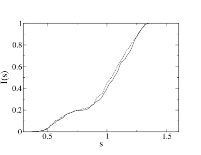
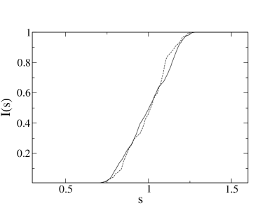
Figure 5: Integrated level spacing distribution for $U(\phi)$ (solid line) and integrated distribution of $G(\phi)$ for $\phi$ uniformly distributed random variable (dashed line) for $N=431$ (left) and $N=5867$ (right).

Appendix

Let us define $\beta_{k,N}$ by

$$e(\beta_{k,N})=e_{N}\left(A^{2}\sum_{r=1}^{A^{-1}k}r^{2}-\frac{Ak}{N}\sum_{r=1}^{N}r^{2}\right)\frac{1}{\sqrt{N}}\sum_{\nu=0}^{N-1}e_{N}\left(Ak\nu^{2}+(A+k)k\nu\right).$$ (30)

It can be shown that the variable $\xi_{j}:=\sqrt{N}\langle\varphi_{j}^{(0)}|\Delta|\varphi_{j}^{(0)}\rangle$ is equal to $\xi_{j}=h(A^{-1}j/N)$, where $h$ is the 1-periodic function

$$h(x)=\sum_{k\in{\mathbb{Z}}}\widehat{\Delta}_{-k}e(kx+\beta_{k,N}),$$ (31)

where $\widehat{\Delta}_{0}=0$, $\widehat{\Delta}_{k}=i/2\pi k$ ($k\neq 0$) are the Fourier coefficients of $\Delta(\phi)$. For $N$ prime, the spectrum of $U_{0}(\Phi_{\alpha})$ is totally rigid [18], that is $\theta^{(0)}_{j}=2\pi j/N+C_{N}$ for $j=1,\ldots,N$, where $C_{N}$ is some overall shift. The corresponding level spacing distribution is hence $P^{(0)}(s)=\delta(s-1)$. For $\epsilon$ small enough, the perturbation does not change the ordering of the levels. The level spacing distribution $P(s)$ for the $\theta_{j}$ is then given by the distribution of the $(N/2\pi)(\theta_{j}-\theta_{j-1})\approx 1+\epsilon\sqrt{N}(\xi_{j}-\xi_{j-1})$, which is equal to $G(A^{-1}j/N)$, where $G$ is the function defined by

$$G(\phi)=1+\epsilon\sqrt{N}\sum_{k\in{\mathbb{Z}}}\widehat{\Delta}_{-k}\,e(\beta_{k,N})\left[1-e_{N}(-A^{-1}k)\right]\,e(k\phi).$$ (32)

For random $j\in\{1,\ldots,N\}$ and $N$ large the distribution of $P(s)$ is asymptotically given by the distribution of $G(\phi)$ where $\phi$ is now a uniformly distributed random variable in $[0,1)$. The variance of the above distribution is $(2\epsilon\sqrt{N})^{2}\sum_{k\in{\mathbb{Z}}}|\widehat{\Delta}_{k}|^{2}\sin^{2}\left(\pi A^{-1}k/N\right)=\epsilon^{2}A^{-1}(1-A^{-1}/N)$, provided we choose $A^{-1}\in[0,N-1]$.

References

[1]
Berry MV and Tabor M 1977 Proc Roy Soc A 356 375
[2]
Bohigas O, Giannoni M-J and Schmit C 1984 Phys Rev Lett52 1
[3]
Haake F 2001 Quantum Signatures of Chaos (Berlin: Springer)
[4]
Bogomolny E, Gerland U and Schmit C 1999 Phys. Rev. E 59 R1315
[5]
Casati G and Prosen T 1999 Quantum chaos in triangular billards
unpublished
[6]
Bogomolny E, Gerland U and Schmit C 2001 Eur Phys J B 19 121
[7]
Bogomolny E, Giraud O and Schmit C 2001 Comm Math Phys222 327
[8]
Gorin T and Wiersig J 2003 Phys Rev E 68 065205(R)
[9]
Berry MV, Balazs NL, Tabor MA and Voros A 1979 Ann Phys122 26
[10]
Hannay JH and Berry MV 1980 Phys D 1 267
[11]
Izrailev FM 1986 Phys Rev Lett56 541
[12]
Bouzouina A and De Bièvre S 1996 Comm Math Phys178 83
[13]
Casati G and Prosen T Phys Rev Lett 2002 85 4261
[14]
Bogomolny E, Georgeot B, Giannoni M-J and Schmit C 1997
Phys Rep291 219
[15]
Bogomolny E and Schmit C 2004 preprint arXiv nlin.CD/0312057
[16]
Aurich R and Marklof J unpublished
[17]
Keppeler S, Marklof J and Mezzadri F 2001 Nonlinearity14 719
[18]
Marklof J and Rudnick Z 2000 GAFA10 1554
[19]
Bäcker A and Haag G 1999 J Phys A 32 L393
[20]
Haag G and Keppeler S 2002 Nonlinearity15 65
[21]
Keppeler S 2003 Spinning particles: semiclassics and spectral statistics
(Berlin: Springer)