Adaptive Synchronization in Coupled Dynamic Networks

Abstract

This paper studies synchronization in coupled nonlinear dynamic networks with unknown parameters. Adaptation can be added to one or several elements in the network, while preserving the global synchronization conditions derived in [22, 26]. This implies that new nodes can be added to the network without prior knowledge of the individual dynamics, and that nodes in an existing network have the ability to recover dynamic information if temporarily lost. In addition, when the individual elements feature sufficiently rich stable dynamics , as e.g. in the case of oscillators, then adaptation actually leads to an exact estimation of the unknown parameters. Different kinds of “leaders” are also discussed in this context - one type of leader can specify overall trajectories for the network, while another can concurrently specify dynamic parameters.

1 INTRODUCTION

While the study of synchronization of coupled dynamic systems has a long history [20, 23], it is still an extremely active research topic [2, 4, 8, 9, 11, 18, 19, 24, 25]. In two recent papers [22, 26], we proposed a new theoretical analysis tool, which we called Partial Contraction Theory, which is based on Contraction concept [13]. We used Partial Contraction Theory to analyze the collective behaviors of dynamic networks with arbitrary size and general connectivity. Synchronization conditions were derived for networks with diffusion-like couplings, which essentially require the network to be connected, the maximum eigenvalue of the uncoupled Jacobian matrix to be upper bounded, and the coupling strengths to exceed a threshold.

In this paper, we extend the results in [22, 26] to coupled networks with adaptation. We show that synchronization still occurs under very similar conditions if adaptation is added to one or more than one elements in a network. Estimated parameters will converge to real values if the stable system behaviors are sufficiently rich or persistently exciting, which is the case when the individual elements are oscillators, for instance. This result is conceptually new as it differs with most existing adaptation models, in the sense that the adaptation here only adds to a small part of the network, and the target behavior is synchronization rather than an explicit desired trajectory. Imagine for instance that some elements in a network lose the normal values of some parameters. They can recover the losing information from the rest of the network, as long as there are still elements holding this information. The nodes holding the real parameters can be considered “knowledge-based leaders”. They differ with the usual “power-based” leaders or virtual leaders such as those in e.g.  [8, 11] and [22, 26], which specify desired trajectories for the network by unidirectionally coupling to it. With adaptation, we can also add new nodes into a network without knowing the dynamic properties of the nodes already in the network.

Section 2 briefly reviews Contraction and Partial Contraction Theories, and the main results we derived for synchronization. Adaptation for two coupled systems is studied in Section 3, and the results are extended to general coupled networks in Section 4. Brief concluding remarks are offered in Section 5.

2 Synchronization in Coupled Networks

2.1 Graph Theory Preliminaries

Let us first introduce some basic Graph Theory concepts [3, 6, 15] which will be used in the rest of the paper.

A graph $G$ is composed of a set of $n$ nodes and a set of $\tau$ links. If there is a direction of flow associated with each link, $G$ is called a directed graph, otherwise it is undirected. $G$ is connected if any two nodes inside are linked by a path. The components of the adjacency matrix ${\bf A}(G)\in\mathbb{R}^{n\times n}$ are defined as $[{\bf A}]_{ij}=1$, for an undirected graph if there is a link connecting nodes $j$ and $i$, and for a directed graph if there is a link from node $j$ to node $i$, and as $[{\bf A}]_{ij}=0$ otherwise. The valency matrix ${\bf D}(G)\in\mathbb{R}^{n\times n}$ is a diagonal matrix with $[{\bf D}]_{ii}=\sum_{j=1}^{n}a_{ij}$. The matrix ${\bf L}(G)={\bf D}-{\bf A}$ is the Laplacian matrix, which is symmetric and positive semi-definite if $G$ is undirected. Its second minimum eigenvalue $\lambda_{2}({\bf L})\$ is the algebraic connectivity, which is zero if and only if $G$ is not connected. The first eigenvalue is always zero, corresponding to the eigenvector $[1,1,\ldots,1]^{T}$.

Assign an arbitrary orientation $\sigma$ to an undirected graph $G$. We get the incidence matrix $={\bf D}(G^{\sigma})\in\mathbb{R}^{n\times\tau}$. For each oriented link $k$ which starts from node $i$ and ends at node $j$, $[{\bf D}]_{ik}=1$ and $[{\bf D}]_{jk}=-1$. All the other entries of ${\bf D}$ are equal to $0$. Moreover,

$${\bf L}(G)={\bf D}(G^{\sigma})\ {\bf D}^{T}(G^{\sigma})$$

If the graph is weighted, we have the weighted Laplacian matrix

$${\bf L}_{\bf\mathcal{K}}\ =\ {\bf D}\ {\bf\mathcal{K}}\ {\bf D}^{T}$$

where $\ {\bf\mathcal{K}}\in\mathbb{R}^{\tau\times\tau}\$ is a diagonal matrix with the $k^{\rm{th}}$ diagonal entry $\ [{\bf\mathcal{K}}]_{k}={\bf K}_{ij}\$ corresponding to the weight of the $k^{\rm{th}}$ link. If ${\bf K}_{ij}\in\mathbb{R}^{m\times m}$ is a matrix, ${\bf\mathcal{K}}$ is block diagonal. Similarly ${\bf D}$ has block entries ${\bf I}$, $-{\bf I}$ and ${\bf 0}$.

2.2 Contraction and Partial Contraction Theories

In two recent papers [22, 26], we studied synchronization behaviors of coupled dynamic networks. Here we briefly introduce the theoretical analysis tools.

Contraction Theory [13]: Consider a nonlinear system $\dot{{\bf x}}={\bf f}({\bf x},t)$ where we assume ${\bf f}({\bf x},t)$ is continuously differentiable. Consider a virtual displacement $\delta{\bf x}$ between two neighboring solution trajectories. We have

$$\frac{d}{dt}({\delta{\bf x}}^{T}{\delta{\bf x}})\ =\ 2\ {\delta{\bf x}}^{T}\frac{\partial{\bf f}}{\partial{\bf x}}\ {\delta{\bf x}}\ \leq\ 2\ \lambda_{max}\ {\delta{\bf x}}^{T}{\delta{\bf x}}$$

where $\ \lambda_{max}({\bf x},t)\$ is the largest eigenvalue of the symmetric part of the Jacobian matrix $\ \partial{\bf f}/\partial{\bf x}\$. Hence, if $\ \lambda_{max}({\bf x},t)\$ is uniformly strictly negative, any infinitesimal length $\ \|\delta{\bf x}\|\$ converges exponentially to zero. By path integration at fixed time, this implies in turn that all the solutions converge exponentially to a single trajectory, independently of the initial conditions.

More generally, consider a coordinate transformation ${\delta{\bf z}}={\bf\Theta}\delta{\bf x}$ where ${\bf\Theta}({\bf x},t)$ is a uniformly invertible square matrix. We have

$$\frac{d}{dt}({\delta{\bf z}}^{T}{\delta{\bf z}})\ =\ 2\ {\delta{\bf z}}^{T}\ (\dot{{\bf\Theta}}+{\bf\Theta}\frac{\partial{\bf f}}{\partial{\bf x}}){\bf\Theta}^{-1}\ \delta{\bf z}$$

so that exponential convergence of $\|\delta{\bf z}\|$ to zero is guaranteed if the generalized Jacobian matrix

$${\bf F}=(\dot{\bf\Theta}+{\bf\Theta}\frac{\partial{\bf f}}{\partial{\bf x}}){\bf\Theta}^{-1}$$

is uniformly negative definite. Again, this implies in turn that all the solutions of the original system converge exponentially to a single trajectory, independently of the initial conditions. Such a system is called contracting .

Partial Contraction Theory [22, 26]: Consider a nonlinear system in the form $\dot{\bf x}\ =\ {\bf f}({\bf x},{\bf x},t)$. Consider the virtual, observer-like auxiliary system

$$\dot{\bf y}\ =\ {\bf f}({\bf y},{\bf x},t)$$

and assume that this system is contracting. By construction, $\ {\bf y}(t)={\bf x}(t)$ is a particular solution of the ${\bf y}$-system. Thus, if another particular solution of the ${\bf y}$-system verifies a smooth specific property, then all trajectories of the ${\bf x}$-system verify this property exponentially. Such a ${\bf x}$-system is called partially contracting.

2.3 Synchronization of Coupled Networks

In this section, we list two main results in [22, 26], both of which will be extended through the rest of the paper.

Two Coupled Systems: Consider the coupled systems

$$\begin{cases}\ \dot{\bf x}_{1}\ =\ {\bf h}({\bf x}_{1},t)\ +\ {\bf g}({\bf x}_{1},{\bf x}_{2},t)\\ \ \dot{\bf x}_{2}\ =\ {\bf h}({\bf x}_{2},t)\ +\ {\bf g}({\bf x}_{1},{\bf x}_{2},t)\end{cases}$$ (1)

where ${\bf x}_{1}$, ${\bf x}_{2}\in\mathbb{R}^{m}$ are the state vectors, and ${\bf g}$ could be any combination of ${\bf x}_{1},{\bf x}_{2}$ and $t$.

Theorem 1

If function ${\bf h}$ in (1) is contracting based on a constant ${\bf\Theta}$, ${\bf x}_{1}$ and ${\bf x}_{2}$ will converge to each other exponentially, regardless of the initial conditions.

The proof is based on the auxiliary system

$$\dot{\bf y}\ =\ {\bf h}({\bf y},t)\ +\ {\bf g}({\bf x}_{1}(t),{\bf x}_{2}(t),t)$$

which is contracting and has two particular solutions ${\bf y}={\bf x}_{1}$ and ${\bf y}={\bf x}_{2}$.

Coupled Networks: Consider a coupled network containing $n$ elements

$$\dot{\bf x}_{i}={\bf f}({\bf x}_{i},t)+\sum_{j\in{\mathcal{N}}_{i}}{\bf K}_{ji}\ ({\bf x}_{j}-{\bf x}_{i})\ \ \ \ i=1,\ldots,n$$ (2)

where ${\mathcal{N}}_{i}$ denotes the set of indices of the active links of element $i$, and the couplings are symmetric positive definite, i.e., ${\bf K}_{ji}={\bf K}_{ij}>0$..

Theorem 2

All the elements within the coupled network (2) will reach group agreement exponentially if

• the network is connected

• $\lambda_{max}({\bf J}_{is})$ is upper bounded

• the coupling strengths are strong enough

where ${\bf J}_{is}$ is the symmetric part of the Jacobian $\frac{\partial{\bf f}({\bf x}_{i},t)}{\partial{\bf x}_{i}}$.

The proof is based on the auxiliary system

$$\dot{\bf y}_{i}={\bf f}({\bf y}_{i},t)+\sum_{j\in{\mathcal{N}}_{i}}{\bf K}_{ji}\ ({\bf y}_{j}-{\bf y}_{i})-\ {\bf K}_{0}\ \sum_{j=1}^{n}({\bf y}_{j}{-\bf x}_{j}(t))$$

which is contracting for appropriate choices of the constant matrix ${\bf K}_{0}>0$. All solutions of (2) thus verify the smooth specific property $\ {\bf x}_{1}=\cdots={\bf x}_{n}\$ exponentially.

In fact, we can express the synchronization condition more specifically as

$$\lambda_{m+1}({\bf L}_{\bf\mathcal{K}})\ >\ \max_{i}\lambda_{max}({\bf J}_{is})\ \ \ \ \ \mathrm{uniformly}$$ (3)

where ${\bf L}_{\bf\mathcal{K}}$ is the weighted Laplacian matrix with each weight corresponding to the coupling strength of that link.

In addition, the coupling forces in a network can be more general, such as uni-directional, positive semi-definite, or nonlinear.

Note that the condition (3) is always true if ${\bf J}_{is}\leq 0$ and the network is connected. For example, assuming ${\bf f}({\bf x}_{i},t)=0$, system (2) represents a schooling or flocking model [22] which provides an effective distributed solution for group agreement problem [8, 11, 18] or rendezvous problem [1, 12].

3 Two Coupled Systems with Adaptation

Consider two coupled systems as in (1), but assume that a parameter vector ${\bf a}$ is unknown to the second system. To guarantee state convergence, we generate an estimated parameter $\hat{\bf a}$ through an adaptation mechanism. Specifically, the ${\bf x}_{2}$ dynamics is replaced by

$$\dot{\bf x}_{2} = {\bf h}({\bf x}_{2},\hat{\bf a},t)\ +\ {\bf g}({\bf x}_{1},{\bf x}_{2},t)$$ (4)

$$\dot{\hat{\bf a}} = {\bf P}{\bf W}^{T}({\bf x}_{2},t)\tilde{\bf x},\ \ \ \ \tilde{\bf x}={\bf x}_{1}-{\bf x}_{2}$$

with constant symmetric ${\bf P}>0$ and ${\bf W}({\bf x}_{2},t)$ defined as

$${\bf h}({\bf x}_{2},\hat{\bf a},t)\ =\ {\bf h}({\bf x}_{2},{\bf a},t)\ +\ {\bf W}({\bf x}_{2},t)\tilde{\bf a}$$

with $\ \tilde{\bf a}=\hat{\bf a}-{\bf a}\$. A similar adaptive technique was used in [13, 14], but is generalized here in the sense that the couplings are bidirectional. The system structure is illustrated in Figure 1.

Figure 1: The structure of two coupled systems with adaptation.

Theorem 3

In system (4), $\tilde{\bf x}$ converges to $0$ asymptotically if ${\bf x}_{1}$ is bounded and ${\bf h}$ is contracting.

Proof: Define the Lyapunov function

$$V = \frac{1}{2}\ (\ \tilde{\bf x}^{T}\tilde{\bf x}\ +\ \tilde{\bf a}^{T}{\bf P}^{-1}\tilde{\bf a}\ )\ >\ 0$$

$$\dot{V} = \tilde{\bf x}^{T}\ (\ {\bf h}({\bf x}_{1},{\bf a},t)\ -\ {\bf h}({\bf x}_{2},{\bf a},t)\ )$$

$$= \tilde{\bf x}^{T}\ \int_{0}^{1}\frac{\partial{\bf h}}{\partial{\bf x}}({\bf x}_{2}+\chi\tilde{\bf x})d\chi\ \tilde{\bf x}\ \leq\ 0$$

The boundedness of ${\bf x}_{1}$ implies that of ${\bf x}_{2}$. Assuming all the functions are smoothly differentiable, the boundedness of $\ddot{V}$ can be concluded since all the states including ${\bf a}$ are bounded. According to Barbalat’s lemma [21], $\dot{V}$ and therefore $\tilde{\bf x}$ tends to $0$ asymptotically. $\Box$

Note that $\dot{\hat{\bf a}}$ also tends to $0$. Furthermore, since $\ddot{\tilde{\bf x}}$ is also bounded, we have the asymptotic convergence of $\dot{\tilde{\bf x}}$ to zero, which leads to the convergence of ${\bf W}({\bf x}_{2},t)\tilde{\bf a}$ to zero. In particular [21], if

$$\exists\ \alpha>0,T>0,\ \ \forall t\geq 0\ \ \int_{t}^{t+T}{\bf W}^{T}{\bf W}dr\ \geq\ \alpha{\bf I}$$

then $\tilde{\bf a}$ converges to zero asymptotically, too.

The boundedness of ${\bf x}_{1}$ is trivial if ${\bf g}={\bf g}({\bf x}_{1},t)$, which is a classical observer structure with ${\bf x}_{1}$ dynamics independent. If ${\bf g}={\bf g}({\bf x}_{1},{\bf x}_{2},t)$, we have

$$\dot{\bf x}_{1}={\bf h}({\bf x}_{1},{\bf a},t)\ +\ {\bf g}({\bf x}_{1},{\bf x}_{1}-\tilde{\bf x},t)={\bf e}({\bf x}_{1},\tilde{\bf x},t)$$

where $\tilde{\bf x}$ is bounded. Thus the boundedness of ${\bf x}_{1}$ is determined by the Input-to-State Stability [10] of ${\bf e}$.

• Example 3.1

  Consider two coupled FitzHugh-Nagumo (FN) neurons [5, 16, 17], a famous spiking neuron model,

  $$\begin{cases}\ \dot{v}_{1}=v_{1}(\alpha-v_{1})(v_{1}-1)-w_{1}+I+k(v_{2}-v_{1})\\ \ \dot{w}_{1}=\beta v_{1}-\gamma w_{1}\end{cases}$$

  $$\begin{cases}\ \dot{v}_{2}=v_{2}(\hat{\alpha}-v_{2})(v_{2}-1)-w_{2}+\hat{I}+k(v_{1}-v_{2})\\ \ \dot{w}_{2}=\hat{\beta}v_{2}-\hat{\gamma}w_{2}\end{cases}$$

  where $v$ is the membrane potential and $I$ external stimulation current. We have ${\bf x}=\left[\begin{array}[]{cc}v&w\end{array}\right]^{T}$, ${\bf a}=\left[\begin{array}[]{cccc}\alpha&I&\gamma&\beta\end{array}\right]^{T}>0$ and

  $${\bf h}({\bf x},{\bf a},t)=\left[\begin{array}[]{c}v(\alpha-v)(v-1)-w+I-2kv\\ \beta v-\gamma w\end{array}\right]$$

  which is contracting if the coupling gain $k$ is larger than an explicit threshold [22]. The adaptive law is thus

  $$\dot{\hat{\bf a}}\ =\ {\bf P}{\bf W}^{T}\tilde{\bf x}$$

  with

  $${\bf W}\ =\ \left[\begin{array}[]{cccc}v_{2}^{2}-v_{2}&1&0&0\\ 0&0&-w_{2}&v_{2}\end{array}\right]$$

  Note that although the diffusion couplings are only based on variable $v$, full-state feedback is needed for adaptation in this case. See Appendix 6.1 for the boundedness proof. The simulation result is illustrated in Figure 2. $\Box$

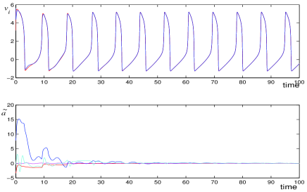
Figure 2: Simulation result of Example 3.1. The real parameters are $\ \alpha=5.32,\beta=3,\gamma=0.1\$ and $\ I=20\$. The coupling gain $\ k=15\$. The matrix $\ {\bf P}=\mathrm{diag}\{0.6,30,0.002,0.4\}\$. All initial conditions are chosen arbitrarily. The plots are (a) states $v_{i}$ versus time, (b) estimator error $\tilde{\bf a}$ versus time.

4 Adaptation in Coupled Networks

4.1 Basic Results

Consider now the coupled network (2). We show that similar synchronization conditions as those in Theorem 2 can be derived if adaptation is added.

For simplicity, we assume that the couplings are bidirectional, which means the corresponding graph is undirected, and $\ {\bf K}_{ji}={\bf K}_{ij}={\bf K}_{k}\$ with $k$ denoting the $k^{th}$ link $(i,j)$. We also assume that each coupling gain is symmetric positive definite, that is, $\ {\bf K}_{k}^{T}={\bf K}_{k}>0\$. Assume now that the uncoupled dynamics $\ {\bf f}({\bf x}_{i},t)={\bf f}({\bf x}_{i},{\bf a},t)\$ contains a parameter set ${\bf a}$ which is unknown to an arbitrary node $\varsigma$. We then use the estimated parameter $\hat{\bf a}$ in $\varsigma$, with an adaptive law based on the local “coupling forces”

$$\dot{\hat{\bf a}}\ =\ {\bf P}{\bf W}^{T}({\bf x}_{\varsigma},t)\sum_{j\in{\mathcal{N}}_{\varsigma}}{\bf K}_{j\varsigma}\ ({\bf x}_{j}-{\bf x}_{\varsigma})$$ (5)

where ${\bf P}$ and ${\bf W}({\bf x}_{\sigma},t)$ are the same as those defined in (4). The network structure is illustrated in Figure 3. Note that the adaptation only uses feedback from the connected neighbors.

Figure 3: Coupled network with adaptation

To prove convergence, we define a Lyapunov function

$$V=\frac{1}{2}\ (\ {\bf x}^{T}{\bf L}_{\bf\mathcal{K}}{\bf x}\ +\ \tilde{\bf a}^{T}{\bf P}^{-1}\tilde{\bf a}\ )$$

where $\ {\bf L}_{\bf\mathcal{K}}={\bf D}{\bf\mathcal{K}}{\bf D}^{T}\$ is the weighted Laplacian matrix, and each weight corresponds to the coupling strength of that link. ${\bf L}_{\bf\mathcal{K}}$ is symmetric positive semi-definite since ${\bf\mathcal{K}}$ is symmetric positive definite. We show that

$$\dot{V} = {\bf x}^{T}{\bf L}_{\bf\mathcal{K}}\dot{\bf x}\ +\ \tilde{\bf a}^{T}{\bf P}^{-1}\dot{\hat{\bf a}}$$

$$= {\bf x}^{T}{\bf L}_{\bf\mathcal{K}}\ (\ \left[\begin{array}[]{c}{\bf f}({\bf x}_{1},{\bf a},t)\\ \ldots\\ {\bf f}({\bf x}_{n},{\bf a},t)\end{array}\right]-{\bf L}_{\bf\mathcal{K}}{\bf x}\ )$$

$$= {\bf x}^{T}\ {\bf D}{\bf\mathcal{K}\Lambda}{\bf D}^{T}\ {\bf x}-{\bf x}^{T}\ {\bf L}_{\bf\mathcal{K}}^{2}\ {\bf x}$$

$$= {\bf x}^{T}\ (\ {\bf L}_{\bf\mathcal{K}\Lambda}-{\bf L}_{\bf\mathcal{K}}^{2}\ )\ {\bf x}$$

where

$${\bf L}_{\bf\mathcal{K}\Lambda}^{T}\ =\ {\bf L}_{\bf\mathcal{K}\Lambda}\ =\ {\bf D}\ ({\bf\mathcal{K}}{\bf\Lambda})_{s}\ {\bf D}^{T}$$

The matrix ${\bf\Lambda}\in\mathbb{R}^{\tau\times\tau}\$ is a block diagonal matrix with the $k^{\rm{th}}$ diagonal entry

$$[{\bf\Lambda}]_{k}=\int_{0}^{1}\frac{\partial{\bf f}}{\partial{\bf x}}({\bf x}_{j}+\chi({\bf x}_{i}-{\bf x}_{j}))\ d\chi$$

corresponding to the $k^{\rm{th}}$ link, which has been assigned with an arbitrary orientation by incidence matrix ${\bf D}$, for instance from node $i$ to node $j$. The matrix $({\bf\mathcal{K}}{\bf\Lambda})_{s}\$, the symmetric part of $\ {\bf\mathcal{K}}{\bf\Lambda}\$, is also a block diagonal matrix with $k^{\rm{th}}$ diagonal entry $\ [({\bf\mathcal{K}}{\bf\Lambda})_{s}]_{k}=({\bf K}_{k}[{\bf\Lambda}]_{k})_{s}\$.

Lemma 1

The matrix $\ {\bf L}_{\bf\mathcal{K}\Lambda}-{\bf L}_{\bf\mathcal{K}}^{2}\$ is negative semi-definite if

$$\frac{\lambda_{m+1}^{2}({\bf L}_{\bf\mathcal{K}})}{\lambda_{n}({\bf L})}>\max_{k}\lambda_{max}({\bf K}_{k}[{\bf\Lambda}]_{k})_{s}$$ (7)

See Appendix 6.2 for the proof.

Lemma 2

Given any vector ${\bf x}=[{\bf x}_{1}^{T},{\bf x}_{2}^{T},\ldots,{\bf x}_{n}^{T}]^{T}$. For a coupled network, if the condition (7) is true,

$${\bf x}^{T}\ (\ {\bf L}_{\bf\mathcal{K}\Lambda}-{\bf L}_{\bf\mathcal{K}}^{2}\ )\ {\bf x}=0$$

if and only if $\ {\bf x}_{1}={\bf x}_{2}=\cdots={\bf x}_{n}$. See Appendix 6.3 for the proof.

Theorem 4

For a connected dynamic network (2) with adaptation (5) adding to an arbitrary node $\varsigma$, the states of all the elements will converge together asymptotically if the condition (7) is true and all the states are bounded.

Proof: Similar to the proof of Theorem 3, if all the states are bounded, we can conclude the boundedness of $\ddot{V}$, which then leads to the asymptotically convergence of $\dot{V}$ to zero if the condition (7) is true. With Lemma 2, this implies immediately that $\ {\bf x}_{1}={\bf x}_{2}=\cdots={\bf x}_{n}$. $\Box$

Remarks:

$\bullet$ Condition (7) in Lemma 1 is in fact very similar to those given in Theorem 2. If $\lambda_{max}({\bf K}_{k}[{\bf\Lambda}]_{k})_{s}$ is positive, to guarantee synchronization one needs a connected network, an upper bounded $\ \lambda_{max}({\bf K}_{k}[{\bf\Lambda}]_{k})_{s}$, and strong enough coupling strength ${\bf\mathcal{K}}$. This result thus implies that adaptation (5) will not significantly change the network’s synchronization ability.

Assuming $m=1$ and all the coupling strengths $\ {\bf K}_{k}=\kappa\$, a sufficient synchronization condition for a coupled network without adaptation is

$$\kappa_{1}\ >\ \frac{\max_{i}{\bf J}_{is}}{\lambda_{2}({\bf L})}$$

while it is

$$\kappa_{2}\ >\ \frac{\lambda_{n}({\bf L})}{\lambda_{2}({\bf L})}\ \frac{\max_{i}{\bf J}_{is}}{\lambda_{2}({\bf L})}$$

with adaptation. Here $\ {\bf J}_{is}=(\partial{\bf f}/\partial{\bf x}_{i})_{s}$.

$\bullet$ When the coupling gains are only positive semi-definite, extra restrictions have to be added to the uncoupled system dynamics to guarantee globally stable synchronization, similarly to the fixed-parameters result in [26]. See Appendix 6.3 for details.

$\bullet$ Theorem 4 requires the states to be bounded. Boundedness can be shown following the same steps as we did in Section 3. In fact, since $\dot{V}\leq 0$, we know that $\tilde{\bf a}$ and $\forall k$, $\tilde{\bf x}_{k}={\bf x}_{i}-{\bf x}_{j}$ are bounded. Thus the boundedness of the states are determined by the Input-to-State Stability of the system

$$\dot{\bf x}_{i}={\bf f}({\bf x}_{i},t)+{\bf u}_{i}$$

Convergence of the estimated parameter set $\hat{\bf a}$ can also be concluded with the same analysis as that in Section 3.

$\bullet$ The result of Theorem 4 still holds if the parameter set ${\bf a}$ is unknown to multiple nodes and adaptations are added to these nodes simultaneously. This can be shown using the Lyapunov-like function

$$V=\frac{1}{2}\ (\ {\bf x}^{T}{\bf L}_{\bf\mathcal{K}}{\bf x}\ +\ \sum_{i}\tilde{\bf a}_{i}^{T}{\bf P}^{-1}_{i}\tilde{\bf a}_{i}\ )$$

The nodes holding the real parameters can thus be considered as “knowledge-based” leaders, which are different from usual “power-based” leaders [8, 11, 22, 26], which specify desired trajectories for the network by unidirectionally coupling to it. At the limit all nodes could be adaptive, although they may then converge to any odd parameter set $-$ while all states will converge together, the desired individual behaviors (such as oscillations) may not be preserved depending on initial conditions. Note that both “power” and “knowledge” leaders may be virtual.

$\bullet$ Note that in Lemma 2 the ${\bf x}_{i}$ may actually tend to zero together. We should exclude this possibility, and the possibility that any component of ${\bf x}_{i}$ converges to zero, with dynamic analysis $-$ for instance by showing that zero is an unstable state.

• Example 4.1

  Consider a group of FN neurons connected in a general network

  $$\begin{cases}\displaystyle\ \dot{v}_{i}=v_{i}(\alpha-v_{i})(v_{i}-1)-w_{i}+I+\sum_{j\in{\mathcal{N}}_{i}}k_{ij}(v_{j}-v_{i})\\ \ \dot{w}_{i}=\beta v_{i}-\gamma w_{i}\ \ \ \ \ \ \ \ \ i=1,\ldots,n\end{cases}$$

  Assume that all the parameters are now unknown to the node $\varsigma$. We add adaptation

  $$\dot{\hat{\bf a}}\ =\ {\bf P}{\bf W}^{T}\ \sum_{j\in{\mathcal{N}}_{\varsigma}}\ \left[\begin{array}[]{cc}k_{j\varsigma}&0\\ 0&k_{j\varsigma}\end{array}\right]\ (\ \left[\begin{array}[]{c}v_{j}\\ w_{j}\end{array}\right]-\left[\begin{array}[]{c}v_{\varsigma}\\ w_{\varsigma}\end{array}\right]\ )$$

  with ${\bf W}$ the same as that defined in Example 3.1. Simulation results are illustrated in Figure 4.

  

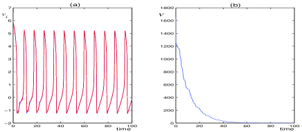
  Figure 4: Simulation results of Example 4. The network contains four FN neurons connected in a two-way ring as Figure 3. The real parameters and the coupling gains are the same as those in Figure 2. The matrix $\ {\bf P}=\mathrm{diag}\{0.06,3,0.0002,0.04\}\$. All the initial conditions are chosen arbitrarily. The plots are (a). states $v_{i}$ versus time, (b).$V$ versus time where, $V=\frac{1}{2}\ (\ {\bf x}^{T}{\bf L}_{\bf\mathcal{K}}{\bf x}\ +\ \tilde{\bf a}^{T}{\bf P}^{-1}\tilde{\bf a}\ )$.

  $\Box$

4.2 Leader Combination

We have mentioned that there can exist different leader roles in a network, ones with power and ones with knowledge. And in fact, these different types of leaders can co-exist. A leader guiding the direction may use state measurements from its neighbors to adapt its parameters to the values of the knowledge leaders.

Consider such a leader-followers network

$$\dot{\bf x}_{0} = {\bf f}({\bf x}_{0},t)$$

$$\dot{\bf x}_{i} = {\bf f}({\bf x}_{i},t)+\sum_{j\in{\mathcal{N}}_{i}}{\bf K}_{ji}({\bf x}_{j}-{\bf x}_{i})+\gamma_{i}{\bf K}_{0i}({\bf x}_{0}-{\bf x}_{i})$$

where $i=1,\ldots,n$, ${\bf x}_{0}$ is the state of the group leader, $\gamma_{i}=0$ or $1$, and ${\mathcal{N}}_{i}$ does not include the links with ${\bf x}_{0}$. Adaptation can be added to any node(s) inside the network, such as

$$\dot{\hat{\bf a}}_{0}\ =\ {\bf P}_{0}{\bf W}^{T}({\bf x}_{0},t)\sum_{i=1}^{n}\gamma_{i}\ {\bf K}_{0i}\ ({\bf x}_{i}-{\bf x}_{0})$$

for the leader, or

$$\dot{\hat{\bf a}}_{i}\ =\ {\bf P}_{i}{\bf W}^{T}({\bf x}_{i},t)(\sum_{j\in{\mathcal{N}}_{i}}{\bf K}_{ji}\ ({\bf x}_{j}-{\bf x}_{i})+\gamma_{i}\ {\bf K}_{0i}\ ({\bf x}_{0}-{\bf x}_{i})\ )$$

for the followers. To prove convergence, we define several Laplacian matrices

$\bullet$ $\bar{\bf L}_{\bf\mathcal{K}}$, the weighted Laplacian of the followers network (excluding both the leader and the links from the leader).

$\bullet$ $\vec{\bf L}_{\bf\mathcal{K}}$, the weighted Laplacian of the leader-followers network, which is not symmetric since we have uni-directional links. Moreover,

$$\vec{\bf L}_{\bf\mathcal{K}}=\left[\begin{array}[]{cc}{\bf 0}&{\bf 0}\\ -{\bf b}&{\bf C}\end{array}\right]$$

where

$${\bf b}=\left[\begin{array}[]{c}\vdots\\ \gamma_{i}\ {\bf K}_{0i}\\ \vdots\end{array}\right],\ \ \ \ {\bf C}=\bar{\bf L}_{\bf\mathcal{K}}+\mathrm{diag}\{\gamma_{i}\ {\bf K}_{0i}\}$$

Note that ${\bf C}$ is symmetric positive definite if the whole leader-followers network is connected.

$\bullet$ ${\bf L}_{\bf\mathcal{K}}$, the weighted Laplacian of the leader-followers network if we consider it as an undirected graph. Thus,

$${\bf L}_{\bf\mathcal{K}}={\vec{\bf L}_{\bf\mathcal{K}}}^{T}+\left[\begin{array}[]{cc}\sum_{i=1}^{n}\gamma_{i}{\bf K}_{0i}&{\bf 0}\\ -{\bf b}&{\bf 0}\end{array}\right]$$

Define

$$V=\frac{1}{2}\ (\ {\bf x}^{T}{\bf L}_{\bf\mathcal{K}}{\bf x}\ +\ \sum_{j}\tilde{\bf a}_{j}^{T}{\bf P}^{-1}_{j}\tilde{\bf a}_{j}\ )$$

where $j$ may be equal to any number from $0$ to $n$. We have

$$\dot{V} = {\bf x}^{T}{\bf L}_{\bf\mathcal{K}}\ (\ \left[\begin{array}[]{c}{\bf f}({\bf x}_{1},{\bf a},t)\\ \ldots\\ {\bf f}({\bf x}_{n},{\bf a},t)\end{array}\right]-\vec{\bf L}_{\bf\mathcal{K}}{\bf x}\ )$$

$$= {\bf x}^{T}\ (\ {\bf L}_{\bf\mathcal{K}\Lambda}-{\vec{\bf L}_{\bf\mathcal{K}}}^{T}\ \vec{\bf L}_{\bf\mathcal{K}}\ )\ {\bf x}$$

See Appendix 6.5 for the conditions for ${\bf L}_{\bf\mathcal{K}\Lambda}-{\vec{\bf L}_{\bf\mathcal{K}}}^{T}\ \vec{\bf L}_{\bf\mathcal{K}}$ to be negative semi-definite. Following the same proofs as in previous sections, this then implies that all the states ${\bf x}_{j}$, $j=0,1,\ldots,n$ converge together. Parameter convergence conditions are also the same.

5 Concluding Remarks

Coupled networks with adaptation are studied in this paper. We showed that synchronized behaviors can be achieved under similar conditions as we derived in [22, 26], which also guarantees parameter convergence if the stable system behaviors are sufficiently rich. Different kinds of leaders may coexist in the network. Current work includes the applications of adaptive network, and the investigation of coupled networks with distributed controllers.

6 Appendices

6.1 Boundedness of Coupled FN Neurons

For notation simplicity, define $u=I+k(v_{2}-v_{1})$ and $\bar{w}=w/\sqrt{\beta}$. The dynamics of the first neuron changes to

$$\begin{cases}\ \dot{v}_{1}=v_{1}(\alpha-v_{1})(v_{1}-1)-\sqrt{\beta}\bar{w}_{1}+u\\ \ \dot{\bar{w}}_{1}=\sqrt{\beta}v_{1}-\gamma\bar{w}_{1}\end{cases}$$ (9)

Define $\ U=\frac{1}{2}\ (\ v_{1}^{2}\ +\ \bar{w}_{1}^{2}\ )$,

$$\dot{U}=-(v_{1}-\alpha)(v_{1}-1)v_{1}^{2}\ -\ \gamma\bar{w}_{1}^{2}\ +\ uv_{1}$$

Since $u$ is bounded, there must exist a large but bounded number $v_{0}>0$, $\forall\ |v_{1}|>v_{0}$, $\dot{U}<0$. We denote the region $|v_{1}|\leq v_{0}$ as $\Omega$.

If the system (9) starts inside $\Omega$, since the dynamics of $\bar{w}_{1}$ is linear and strictly stable, $v_{1}$ and $\bar{w}_{1}$ are always bounded as long as the system stays inside $\Omega$. In fact,

$$|\bar{w}_{1}(t)| = |(\ \bar{w}_{1}(0)+\int_{0}^{t}\sqrt{\beta}v_{1}(t)e^{\gamma t}dt\ )\ e^{-\gamma t}|$$

$$\leq |\bar{w}_{1}(0)|e^{-\gamma t}\ +\ v_{0}\frac{\sqrt{\beta}}{\gamma}(1-e^{-\gamma t})$$

Thus, for any initial condition $|\bar{w}_{1}(0)|>v_{0}\frac{\sqrt{\beta}}{\gamma}$, we have $|\bar{w}_{1}(t)|\leq|\bar{w}_{1}(0)|$, which implies that the bound of $|\bar{w}_{1}(t)|$ inside $\Omega$ is $\max(v_{0}\frac{\sqrt{\beta}}{\gamma},|\bar{w}_{1}(0)|)$.

Suppose that at some moment, the system leaves $\Omega$ through point $(v_{0}\ \bar{w}_{out})$. Since $\dot{U}<0$ outside $\Omega$, $v_{1}^{2}(t)$ and $\bar{w}_{1}^{2}(t)$ will be both bounded by $v_{0}^{2}+\bar{w}_{out}^{2}$ until the system trajectory re-enters $\Omega$, at which moment we should have $|\bar{w}_{in}|<|\bar{w}_{out}|$. See Figure 5 for an illustration. The proof is similar if the system starts outside $\Omega$.

Figure 5: Illustration of a solution trajectory of the system (9) leaving and re-entering the region $\Omega:\ |v_{1}|\leq v_{0}$.

Thus, ${\bf x}_{1}=\left[\begin{array}[]{cc}v_{1}&w_{1}\end{array}\right]^{T}$ is always bounded, which leads to asymptotic convergence of $\tilde{\bf x}$ to $0$ according to Theorem 3. Moreover, since the two FN neurons synchronize along a limit cycle, the convergence of ${\bf W}({\bf x}_{2},t)\tilde{\bf a}$ to zero implies that of $\tilde{\bf a}$.

6.2 Proof of Lemma ${\bf 1}$

For notation simplicity, we first choose $m=1$. Since

$${\bf L}_{\bf\mathcal{K}\Lambda}-{\bf L}_{\bf\mathcal{K}}^{2}\ =\ {\bf D}\ (\ ({\bf\mathcal{K}\Lambda})_{s}-{\bf\mathcal{K}D}^{T}{\bf D\mathcal{K}}\ )\ {\bf D}^{T}$$

we know that $0$ is always one of its eigenvalues, with the corresponding eigenvector $\ {\bf v}=[1,1,\ldots,1]^{T}\$. Assume that the eigenvalues $\ \lambda_{i}({\bf L}_{\bf\mathcal{K}\Lambda})$, $\lambda_{i}({\bf L}_{\bf\mathcal{K}}^{2})$, $\lambda_{i}({\bf L}_{\bf\mathcal{K}\Lambda}-{\bf L}_{\bf\mathcal{K}}^{2})\$ are all arranged in increasing order for $i=1,2,\ldots,n$. According to Weyl’s Theorem [7], for two Hermitian matrix ${\bf A}$ and ${\bf B}$,

$$\lambda_{k}({\bf A})+\lambda_{1}({\bf B})\ \leq\ \lambda_{k}({\bf A}+{\bf B})\ \leq\ \lambda_{k}({\bf A})+\lambda_{n}({\bf B})$$

for each $k=1,2,\ldots,n$. Thus, we have

$$\lambda_{n-k+1}({\bf L}_{\bf\mathcal{K}\Lambda}-{\bf L}_{\bf\mathcal{K}}^{2})\ \leq\ \lambda_{n}({\bf L}_{\bf\mathcal{K}\Lambda})-\lambda_{k}({\bf L}_{\bf\mathcal{K}}^{2})$$

which implies that, $\forall k>1$, $\lambda_{n-k+1}({\bf L}_{\bf\mathcal{K}\Lambda}-{\bf L}_{\bf\mathcal{K}}^{2})<0$ if

$$\lambda_{n}({\bf L}_{\bf\mathcal{K}\Lambda})\ <\ \lambda_{2}({\bf L}_{\bf\mathcal{K}}^{2})$$ (10)

Therefore, $\lambda_{n}({\bf L}_{\bf\mathcal{K}\Lambda}-{\bf L}_{\bf\mathcal{K}}^{2})=0$, that is, ${\bf L}_{\bf\mathcal{K}\Lambda}-{\bf L}_{\bf\mathcal{K}}^{2}$ is negative semi-definite.

In fact, $\lambda_{2}({\bf L}_{\bf\mathcal{K}}^{2})=\lambda_{2}^{2}({\bf L}_{\bf\mathcal{K}})$. Assume

$$\max_{k}\lambda_{max}({\bf K}_{k}[{\bf\Lambda}]_{k})_{s}\ =\ \bar{\lambda}$$

If $\bar{\lambda}\leq 0$, we have $\lambda_{n}({\bf L}_{\bf\mathcal{K}\Lambda})\leq 0$ and both the conditions (10) and (7) are always true. If $\bar{\lambda}>0$, then

$$\lambda_{n}({\bf L}_{\bf\mathcal{K}\Lambda})\ \leq\ \bar{\lambda}\ \lambda_{n}({\bf L})$$

and the result in Lemma 1 is concluded.

In case $m>1$, we can follow the same proof except that zero eigenvalue here has $m$ multiplicity, and the corresponding eigenvectors $\ \{{\bf v}_{1},{\bf v}_{2},\ldots,{\bf v}_{m}\}\$ are linear combinations of the orthogonal set $\ [{\bf I},{\bf I},\ldots,{\bf I}]^{T}\$ where $\ {\bf I}\in\mathbb{R}^{m\times m}$ is identity matrix.

6.3 Proof of Lemma ${\bf 2}$

For a real symmetric matrix, the state space has an orthogonal basis consisting of all eigenvectors. Without loss generality, we assume such an orthogonal eigenvector set of $\ {\bf L}_{\bf\mathcal{K}\Lambda}-{\bf L}_{\bf\mathcal{K}}^{2}\$ as $\ \{{\bf v}_{1},{\bf v}_{2},\ldots,{\bf v}_{mn}\}$, where $\ [{\bf v}_{1},{\bf v}_{2},\ldots,{\bf v}_{m}]=[{\bf I},{\bf I},\ldots,{\bf I}]^{T}\$ are zero eigenvectors. Therefore for any vector ${\bf x}$, we have ${\bf x}=\sum_{i=1}^{mn}k_{i}{\bf v}_{i}$ and

$${\bf x}^{T}\ (\ {\bf L}_{\bf\mathcal{K}\Lambda}-{\bf L}_{\bf\mathcal{K}}^{2}\ )\ {\bf x}$$

$$= \sum_{i=1}^{mn}k_{i}{\bf v}_{i}^{T}\ (\ {\bf L}_{\bf\mathcal{K}\Lambda}-{\bf L}_{\bf\mathcal{K}}^{2}\ )\ \sum_{i=1}^{mn}k_{i}{\bf v}_{i}$$

$$= \sum_{i=m+1}^{mn}k_{i}{\bf v}_{i}^{T}\ (\ {\bf L}_{\bf\mathcal{K}\Lambda}-{\bf L}_{\bf\mathcal{K}}^{2}\ )\ \sum_{i=m+1}^{mn}k_{i}{\bf v}_{i}$$

$$= \sum_{i=m+1}^{mn}\lambda_{i}k_{i}^{2}{\bf v}_{i}^{T}{\bf v}_{i}$$

where $\lambda_{i}$ is the $i^{th}$ eigenvalue corresponding to the eigenvector ${\bf v}_{i}$, and $\ \lambda_{i}<0$ $\forall i>m$ for a coupled network if the condition (7) is true. Thus, ${\bf x}^{T}\ (\ {\bf L}_{\bf\mathcal{K}\Lambda}-{\bf L}_{\bf\mathcal{K}}^{2}\ )\ {\bf x}=0\$ if and only if $\ {\bf x}=\sum_{i=1}^{m}k_{i}{\bf v}_{i}\$, that is,

$${\bf x}\ =\ [{\bf I},{\bf I},\ldots,{\bf I}]^{T}[k_{1},\ldots,k_{m}]^{T}\ =\ [{\bf x}_{0},{\bf x}_{0},\ldots,{\bf x}_{0}]^{T}$$

where $\ {\bf x}_{0}=[k_{1},\ldots,k_{m}]^{T}$.

6.4 Positive Semi-Definite Couplings

Assume the coupling gain of the $k^{th}$ link is

$${\bf K}_{k}=\left[\begin{array}[]{cc}{\bf K}_{1}&0\\ 0&0\end{array}\right]_{k}$$

where ${\bf K}_{1k}$ is symmetric positive definite and has a common dimension to all links. We divide the uncoupled dynamics ${\bf J}$, and in turn the block diagonal entry of ${\bf\Lambda}$ into the form

$$[{\bf\Lambda}]_{k}=\frac{\partial{\bf f}}{\partial{\bf x}}(\bar{\bf x},t)\ =\ {\bf J}_{k}(\bar{\bf x},t)\ =\ \left[\begin{array}[]{cc}{\bf J}_{11}&{\bf J}_{12}\\ {\bf J}_{21}&{\bf J}_{22}\end{array}\right]_{k}$$

where $\bar{\bf x}$ is a value between the states of two neighboring nodes ${\bf x}_{i}$ and ${\bf x}_{j}$, and each component of ${\bf J}_{k}$ has the same dimension as that of the corresponding part in ${\bf K}_{k}$. Re-define the function $V$ as

$$V=\frac{1}{2}\ (\ {\bf x}^{T}{\bf L}_{\bf\mathcal{K}}{\bf x}\ +\ {\bf x}^{T}{\bf L}_{\bf Y}{\bf x}\ +\ \tilde{\bf a}^{T}{\bf P}^{-1}\tilde{\bf a}\ )$$

where $\ {\bf L}_{\bf Y}={\bf D}{\bf Y}{\bf D}^{T}\$ is a weighted Laplacian based on the same graph as ${\bf L}_{\bf\mathcal{K}}$ but different weights

$${\bf Y}_{k}=\left[\begin{array}[]{cc}0&0\\ 0&{\bf K}_{2}\end{array}\right]_{k}$$

Using a modified adaptive law

$$\dot{\hat{\bf a}}\ =\ {\bf P}{\bf W}^{T}({\bf x}_{\varsigma},t)\sum_{j\in{\mathcal{N}}_{\varsigma}}({\bf K}+{\bf Y})_{j\varsigma}\ ({\bf x}_{j}-{\bf x}_{\varsigma})$$

we can show that

$$\dot{V} = {\bf x}^{T}\ (\ {\bf L}_{\bf(\mathcal{K}+Y)\Lambda}-{\bf L}_{\bf\mathcal{K}}^{2}\ )\ {\bf x}$$

$$= {\bf x}^{T}\ {\bf L}_{\bf(\mathcal{K}+Y)(\Lambda-\bar{\Lambda})}\ {\bf x}\ +\ {\bf x}^{T}\ (\ {\bf L}_{\bf\mathcal{K}\bar{\Lambda}}-{\bf L}_{\bf\mathcal{K}}^{2}\ )\ {\bf x}$$

where we define $[\bar{\bf\Lambda}]_{k}\ =\ \left[\begin{array}[]{cc}\bar{\bf J}_{11}&0\\ 0&0\end{array}\right]_{k}$ so that

$$[{\bf\mathcal{K}\bar{\Lambda}}]_{k}\ =\ \left[\begin{array}[]{cc}{\bf K}_{1}\bar{\bf J}_{11}&0\\ 0&0\end{array}\right]_{k}$$

$$[{\bf(\mathcal{K}+Y)(\Lambda-\bar{\Lambda})}]_{k}\ =\ \left[\begin{array}[]{cc}{\bf K}_{1}({\bf J}_{11}-\bar{\bf J}_{11})&{\bf K}_{1}{\bf J}_{12}\\ {\bf K}_{2}{\bf J}_{21}&{\bf K}_{2}{\bf J}_{22}\end{array}\right]_{k}$$

A non-positive $\dot{V}$ can be guaranteed if

$\bullet$ ${\bf L}_{\bf\mathcal{K}\bar{\Lambda}}-{\bf L}_{\bf\mathcal{K}}^{2}\ \leq 0\$, which can be satisfied under similar condition as (7);

$\bullet$ ${\bf(\mathcal{K}+Y)(\Lambda-\bar{\Lambda})}\ <0$, which is true if $\forall\ k$, the symmetric parts of $\ {\bf K}_{1}({\bf J}_{11}-\bar{\bf J}_{11})\$ and $\ {\bf K}_{2}{\bf J}_{22}\$ are both negative definite, and $\ \sigma_{max}({\bf K}_{1}{\bf J}_{12}+{\bf J}_{21}^{T}{\bf K}_{2}^{T})\$ is bounded. An explicit condition can be derived with feedback combination analysis [22, 26].

The rest of the convergence proof are the same as that of positive definite couplings.

6.5 Leader Combination

Similarly to the proof of Lemma 6.2, choose $m=1$ for notational simplicity. It can be shown that $0$ is always one of the eigenvalues of ${\bf L}_{\bf\mathcal{K}\Lambda}-{\vec{\bf L}_{\bf\mathcal{K}}}^{T}\ \vec{\bf L}_{\bf\mathcal{K}}$, which is negative semi-definite if

$$\lambda_{n+1}({\bf L}_{\bf\mathcal{K}\Lambda})\ <\ \lambda_{2}({\vec{\bf L}_{\bf\mathcal{K}}}^{T}\ \vec{\bf L}_{\bf\mathcal{K}})$$

and its only eigendirection for the zero eigenvalue is ${\bf v}=[1,1,\ldots,1]^{T}$. Since

$${\vec{\bf L}_{\bf\mathcal{K}}}^{T}\ \vec{\bf L}_{\bf\mathcal{K}}=\left[\begin{array}[]{cc}{\bf b}^{T}{\bf b}&-{\bf b}^{T}{\bf C}\\ -{\bf C}{\bf b}&{\bf C}^{2}\end{array}\right]$$

we have

$$\lambda_{2}({\vec{\bf L}_{\bf\mathcal{K}}}^{T}\ \vec{\bf L}_{\bf\mathcal{K}})\geq\lambda_{1}({\bf C}^{2})=\lambda_{1}^{2}({\bf C})$$

from the interlacing eigenvalues theorem for bordered matrices [7]. Thus a sufficient condition for synchronization is

$$\lambda_{1}^{2}({\bf C})>\lambda_{n+1}({\bf L}_{\bf\mathcal{K}\Lambda})$$

This condition is equivalent to the three requirements we listed in the first remark in Section 4.1. Note that the connectedness condition refers to the whole network, while the subnetwork containing only the followers may not be connected.

If all the coupling strengths are identical with gain $\kappa$, the synchronization condition is

$$\kappa\ >\ \frac{\lambda_{n+1}({\bf L})\ \max_{i}{\bf J}_{is}}{\lambda_{1}^{2}(\bar{\bf L}+\mathrm{diag}\{\gamma_{i}\})}$$

where $\bar{\bf L}$ is the Laplacian matrix for the subnetwork containing only followers, and ${\bf L}$ for the whole undirected leader-followers network.

The proof is similar for $m>1$.

References

- [1] Ando, H., Oasa, Y., Suzuki, I., and Yamashita, M. (1999) Distributed Memoryless Point Convergence Algorithm for Mobile Robots with Limited Visibility, IEEE Transactions on Robotics and Automation, 818-828
- [2] D’Andrea, R., and Dullerud, G.E. (2003) Distributed Control Design for Spatially Interconnected Systems, IEEE Transactions on Automatic Control, 48(9):1478-1495
- [3] Fiedler, M. (1973) Algebraic Connectivity of Graphs, Czechoslovak Mathematical Journal, 23(98): 298-305
- [4] Fierro, R., Song, P., Das, A., and Kumar, V. (2002) Cooperative Control of Robot Formations, in Cooperative Control and Optimization: Series on Applied Optimization, Kluwer Academic Press, 79-93
- [5] FitzHugh, R.A. (1961) Impulses and Physiological States in Theoretical Models of Nerve Membrane, Biophys. J., 1:445-466
- [6] Godsil, C., and Royle, G. (2001) Algebraic Graph Theory, Springer
- [7] Horn, R.A., and Johnson, C.R. (1985) Matrix Analysis, Cambridge University Press
- [8] Jadbabaie, A., Lin, J., and Morse, A.S. (2003) Coordination of Groups of Mobile Autonomous Agents Using Nearest Neighbor Rules, IEEE Transactions on Automatic Control, June, 48:988-1001
- [9] Jadbabaie, A., Motee, N., and Barahona, M. (2004) On the Stability of the Kuramoto Model of Coupled Nonlinear Oscillators, Submitted to the American Control Conference
- [10] Khalil H.K. (1996) Nonlinear Systems, Prentice-Hall
- [11] Leonard, N.E., and Fiorelli, E. (2001) Virtual Leaders, Artificial Potentials and Coordinated Control of Groups, 40th IEEE Conference on Decision and Control
- [12] Lin, J., Morse, A., and Anderson, B. (2003) Multi-Agent Rendezvous Problem, Proceedings of the 42nd IEEE Conference on Decision and Control
- [13] Lohmiller, W., and Slotine, J.J.E. (1998) On Contraction Analysis for Nonlinear Systems, Automatica, 34(6)
- [14] Lohmiller, W. (1999) Contraction Analysis of Nonlinear Systems, Ph.D. Thesis, Department of Mechanical Engineering, MIT
- [15] Mohar, B. (1991) Eigenvalues, Diameter, and Mean Distance in Graphs, Graphs and Combinatorics 7:53-64
- [16] Murray, J.D. (1993) Mathematical Biology, Springer-Verlag
- [17] Nagumo, J., Arimoto, S., and Yoshizawa, S. (1962) An Active Pulse Transmission Line Simulating Nerve Axon, Proc. Inst. Radio Engineers, 50:2061-2070
- [18] Olfati-Saber, R., and Murray, R.M. (2003) Consensus Protocols for Networks of Dynamic Agents, American Control Conference, Denver, Colorado
- [19] Pecora, L.M., and Carroll, T.L. (1990) Synchronization in Chaotic Systems, Phys. Rev. Lett., 64:821-824
- [20] Pikovsky, A., Rosenblum, M., and Kurths, J. (2003) Synchronization: A Universal Concept in Nonlinear Sciences, Cambridge University Press
- [21] Slotine, J.J.E., and Li, W. (1991) Applied Nonlinear Control, Prentice-Hall
- [22] Slotine, J.J.E., and Wang, W. (2003) A Study of Synchronization and Group Cooperation Using Partial Contraction Theory, Block Island Workshop on Cooperative Control, Kumar V. Editor, Springer-Verlag
- [23] Strogatz, S. (2003) Sync: The Emerging Science of Spontaneous Order, New York: Hyperion
- [24] Vicsek, T. (2002) The Bigger Picture, Nature, 418:131
- [25] von der Malsburg, C. (1981) The Correlation Theory of Brain Function, Max-Planck-Institut Biophys. Chem., Internal Rep. 81-2, Gttingen FRG
- [26] Wang, W., and Slotine, J.J.E. (2003) On Partial Contraction Analysis for Coupled Nonlinear Oscillators, submitted to Biological Cybernetics