Quasi-Scarred Resonances in a Spiral-Shaped Microcavity

Abstract

We study resonance patterns of a spiral-shaped dielectric microcavity with chaotic ray dynamics. Many resonance patterns of this microcavity, with refractive indices $n=2$ and $3$, exhibit strong localization of simple geometric shape, and we call them quasi-scarred resonances in the sense that there is, unlike the conventional scarring, no underlying periodic orbits. It is shown that the formation of quasi-scarred pattern can be understood in terms of ray dynamical probability distributions and wave properties like uncertainty and interference.

The scar phenomenon, since its advent in a chaotic billiard, has attracted much attention He84 , because it had not been anticipated from the prevailed random matrix theory Bo84 . It is now known that the scarred eigenfunctions show not only strong enhancement along a unstable periodic orbit, but also detail of the stable and unstable manifolds around the periodic orbit Cr02 . This scar effect therefore has been regarded as an important feature of chaotic systems different from random systems. Another important aspect of the scarring effect is its ubiquitous existence; it has been observed in various chaotic systems such as microwave cavity Sr91 , semiconductor quantum well Fr95 , surface wave Ku01 , optical cavities Lee02 ; Re02 , etc.

Recently there is a considerable interest in the light emission from dielectric cavities with chaotic ray dynamics, since many intriguing light emission behaviors take place and are known to be relevant to the underlying chaotic ray dynamics Gm98 . There are several reports of observation of scarred lasing modes in dielectric microcavities of various boundary shapes Lee02 ; Gm02 ; Re02 . The scarred lasing modes generally show good directionality of light emission, the directionality is an important characteristic required for applications to photonic and optoelectric information processing Ch96 . The number of directional beams of the scarred emission from usual microcavities would be more than two because of the discrete symmetry of the boundary geometry and the possibility of interchanging incident and reflected rays on the underlying periodic orbit.

In a remarkable experiment, Chern et al. have successfully observed unidirectional emission in spiral-shaped quantum-well microlasers Ch03 . The unidirectional laser beam is important to arrange easy optical communication between microlasers. The spiral-shaped boundary, in which ray dynamics is chaotic, is given by

$$r(\phi)=R(1+\frac{\epsilon}{2\pi}\phi)$$ (1)

in polar coordinates ($r$, $\phi$), where $R$ is the radius of the spiral at $\phi=0$ and $\epsilon$ is the deformation parameter. Basically, the unidirectionality of the emission beam comes from the special properties of the spiral-shaped boundary geometry which other common cavity designs do not have. They are the absence of any symmetry and the existence of the notch. As mentioned above, the absence of symmetry would be the necessary condition for the unidirectional emission. The notch makes the microcavity show very strong chirality by transmitting or reflecting counterclockwise rotating rays. The bouncing from the notch is inevitable for the rays and would be an essential process for the unidirectional emission. Besides the unidirectionality, it is important and interesting to study how the unique characteristics of the spiral-shaped microcavity appear on resonance patterns.

In this Letter, we investigate the resonance patterns in the spiral-shaped dielectric microcavity. We find that a large number of resonances obtained are strongly localized and that the localized patterns are not supported by any unstable periodic orbit, so we call them quasi-scarred resonances. The existence of quasi-scarred resonances implies that the scarring phenomenon in dielectric microcavities has substantial differences from the conventional scarring in billiard systems. The differences come from inherent characteristics of dielectric cavities such as existence of the critical incident angle for total internal reflection and energy loss by refractive emission. We explain the formation of the quasi-scarred resonances in terms of ray dynamical probability distributions and wave properties like uncertainty and interference. For convenience, we take $\epsilon=0.1$ and $R=1$ in this Letter.

In order to investigate the ray dynamical properties of the spiral-shaped dielectric microcavity, we first consider a uniform ensemble of initial points over the whole phase space $(s,~{}p)$, where $s$ is the boundary arc length from the $\phi=0$ point (see Fig. 4) and its conjugate variable $p$ is given as $p=\sin\theta$, $\theta$ being the incident angle of ray. If the boundary is made by a perfect mirror, the distribution of the points in the phase space at later times would remain uniform (in a random sense) and structureless. However, in the dielectric microcavity, the distribution of the points is, some time later, not uniform but rather structural because the individual ray can suffer energy loss by refractive emission when bouncing from boundary. The amount of the energy loss is determined by the transmission coefficient ${\cal T}(p)$ Ha95 which has a nonzero value in the range of $-p_{c}<p<p_{c}$, where $p_{c}$ is the critical line for total internal reflection and is related to the refractive index $n$ as $p_{c}=\sin\theta_{c}=1/n$, $\theta_{c}$ being the corresponding critical incident angle. This leaky property of rays in the ensemble is described by the survival probability distribution $\tilde{P}(s,p,t)$, the probability with which the ray with $(s,~{}p)$ can survive in the microcavity at a time $t$. With the survival probability distribution $\tilde{P}(s,p,t)$, the energy ${\cal E}(t)$ confined in the microcavity and the escape time distribution $P_{es}(t)$ are expressed as ${\cal E}(t)={\cal E}_{0}\int ds\,dp\,\tilde{P}(s,p,t)$, ${\cal E}_{0}$ being the initial energy, and $P_{es}(t)=\int ds\,dp\,\tilde{P}(s,p,t){\cal T}(p)$, respectively. Since the confined energy decreases by the ray transmission through cavity boundary, we can get a relation,

$$\frac{d{\cal E}(t)}{dt}=-{\cal E}_{0}P_{es}(t).$$ (2)

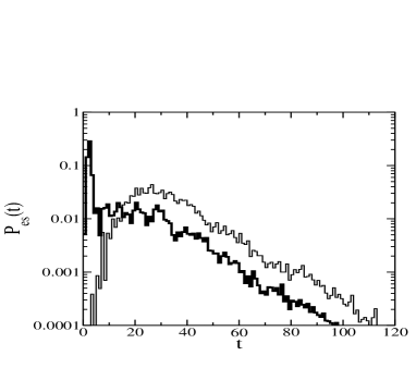
Figure 1: The escape time distributions $P_{es}(t)$ with $n=2$ for two different sets of initial points; the thick and thin lines represent numerical results for Set A and Set B, respectively. The time $t$ is scaled to be the length of ray trajectory when $R=1$.

It is well known that in fully chaotic open systems the escape time distribution $P_{es}(t)$ shows exponential long time behavior, while it becomes power law decay in the KAM systems due to the stickiness of the KAM tori Sc02 . The exponential behavior of $P_{es}(t)$ suggests that $\tilde{P}(s,p,t)$ would have the same phase space distribution after a certain period of time, i.e.,

$$\tilde{P}(s,p,t)=B(t)P_{s}(s,p),$$ (3)

which defines the steady probability distribution $P_{s}(s,p)$ as the stationary part of $\tilde{P}(s,p,t)$. It is obvious from Eq. (2) that the relation in Eq. (3) is equivalent to assuming the exponential time behaviors of ray dynamical distributions such as ${\cal E}(t)$, $\tilde{P}(s,p,t)$, and $P_{es}(t)$. In the case of dielectric microcavities, a numerical justification of the relation in Eq. (3) will be presented below (see Fig. 1). The steady probability distribution $P_{s}(s,p)$ then characterizes the ray dynamical long time behavior. The decay rate $\gamma$, from Eq. (2), can be expressed as

$$\gamma=\int ds\,dp\,P_{s}(s,p){\cal T}(p),$$ (4)

and the ray dynamical near field and far field distributions can be also described by $P_{s}(s,p)$.

For simplicity’s sake, we will concentrate on TM (transverse magnetic) polarization in this Letter. In Fig. 1, the escape time distributions $P_{es}(t)$ are shown for the $n=2$ case. Here, we consider two different sets of $400\times 400$ initial points: one is the uniformly distributed set over the whole phase space (Set A) and the other is the uniformly distributed one in a part of the phase space, $(0<s<s_{max}/2,~{}0.5<p<0.75)$ (Set B), where $s_{max}$ is the total length of the boundary. Note that above $t_{c}\simeq 30$ exponential decay behaviors are shown. The slope of the linear part determines the decay rate $\gamma$. The similar slopes for both Set A and Set B reflect that rays lose their energy through the same process. The details of the process appear in the structure of $P_{s}(s,p)$.

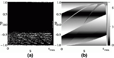
Figure 2: (a) The normalized survival probability distribution $\tilde{P}(s,p,t)$ sampled in the time range of $57<t<60$ for Set A. The white dots represent points whose weight is greater than $0.1$ after normalization. (b) The distance, resulting after 3 bounces, distribution $d(s,p)$. From comparing both figures, it is clear that the partially reflected rays near $-p_{c}$ would make rough triangular trajectories.

Figure 2 (a) shows an approximate $P_{s}(s,p)$ for $n=2$ given by normalizing the $\tilde{P}(s,p,t)$ in the time range of $57<t<60$ for Set A. The structure of the approximate $P_{s}(s,p)$ is almost invariant in other time ranges of the linear part $(t>t_{c})$ and even for Set B. It is clear that the energy loss was mainly caused by tangential emissions just above the critical line ($-p_{c}=-1/2$). So, we can see that the process mentioned above is the way that the ray trajectories first rotate counterclockwise ($p>p_{c}$), then change their rotational direction by reflection on the notch part, and afterwards gradually approach $-p_{c}$. Most of them are emitted out from the microcavity and the remains repeat the same process. The distribution confined to the negative value of $p$ means strong chirality of this spiral-shaped microcavity. The dark tentacular structure in Fig. 2 (a) implies the missing trajectories which are reflected at the notch with $|p|>p_{c}$. In fact, the overall structure presents a part of unstable manifolds, which is typical in open chaotic systems Sc02 . This structure would give important informations about statistical properties of resonances, i.e., far field and near field distribution of resonances would show minima at values corresponding to the missing trajectories.

More direct implication on resonance patterns can arise from the distribution of resulting distance after 3 bounces (Fig. 2(b)), i.e., $d(s,p)=\sqrt{(s_{f}-s)^{2}+(p_{f}-p)^{2}}$ where $(s,~{}p)$ is the initial position and $(s_{f},~{}p_{f})$ being the position after 3 bounces. We note that in Fig. 2 (b) the critical line $p=-p_{c}$ lies on the region of lower $d$ values. Since the rays in the region just above $-p_{c}$ are partially emitted out, the remaining reflected rays would make a rough triangle. As discussed below, the imprint of this fact appears apparently in resonance patterns (see Fig. 3 (a)). Although the $n=3$ case is not presented in the figures, the distance distribution after 5 bounces also shows similar features, implying that the star shape ray trajectories would be responsible for resonance patterns (see Fig. 3 (b)).

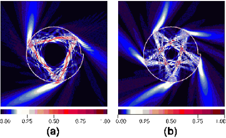
Figure 3: (color). Field intensity plots of quasi-scarred resonances in the spiral-shaped microcavity. (a) $n=2$ and $nkR=(109.70,-0.1128)$. (b) $n=3$ and $nkR=(109.59,-0.1127)$. In figures, the field intensity is normalized by scaling the maximum intensity as one.

Using the boundary element method Wie03 , we obtain resonances around $\mbox{Re}(nkR)\simeq 110$ for the spiral-shaped dielectric microcavity, 24 resonances for $n=2$ and 23 resonances for $n=3$, which are about 25% of the total number of resonances in the concerned range. From the resonances we realize an important fact that the basic localized structures of the resonance patterns are triangular and star shapes for $n=2$ and $3$, respectively, which is consistent with the implication of $P_{s}(s,p)$. Some of these resonances look like strongly scarred eigenfunctions of billiard system, showing strong directional emissions matched to the triangular and star patterns. The $nkR$ values and patterns for whole resonances will be presented elsewhere due to lack of space.

The most clearly localized resonances for $n=2$ and $3$ are shown in Fig. 3. The patterns look like strongly scarred resonances, but there is no exact underlying unstable periodic orbit. Absence of periodic orbits of simple geometry, without bouncing at notch, e.g., triangle and star, is evident by numerical evaluation of $\delta p=p_{i}-p_{f}$ for a closed triangle or star trajectory starting from $(s_{i},p_{i})$ and terminating at $(s_{i},~{}p_{f})$. Moreover nonexistence of periodic orbits of simple geometry can be understood if one know that for the clockwise rotating case the distance between origin and the ray segment always decreases as far as the ray bounces at the curved part of the spiral-shape boundary. We obtain $|\delta p|>\sigma$ for arbitrary $s_{i}$ value, where $\sigma=0.075$ for the triangle trajectory and $\sigma=0.136$ for the star trajectory. Since the localized patterns of resonances are not supported by any unstable periodic orbit, we call them quasi-scarred resonances. The existence of quasi-scarred resonances in dielectric cavities can be understood from the inherent property of dissipative systems, i.e., uncertainty characteristics. Another important result from the resonance pattern analysis is that many resonances are quasi-scarred, e.g., in the present case more than a half are quasi-scarred, while only a small fraction of eigenfunctions are scarred in billiard systems. In practical experiment, this implies that the quasi-scarred lasing emission can be excited easily due to its dominant existence in resonances. In fact, the dominant existence of quasi-scarred resonances can be regarded as a result of the openness of microcavities. In open systems, rather local part of phase space would support resonances(e.g., see Fig. 2(a)) and the resulting individual resonance would show a stong localization whose pattern might be determined by the property of the openness. This is consistent with results, associated with scarred resonances, in various open systems Ku01 ; Kim02

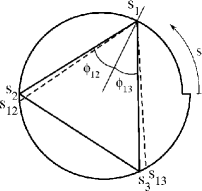
Figure 4: Schematic diagram for quantifying the degree of uncertainty. The trajectory satisfying the Snell’s law, with an incident angle $(\phi_{12}+\phi_{13})/2$, is denoted by dashed lines.

Now, we consider bouncing positions of the triangle formed in quasi-scarred resonances which seem to have a definite dependence on their $\mbox{Re}(nkR)$ values. We assume that the triangle in quasi-scarred resonances has minimum deviation from the ray trajectory governed by the Snell’s law, and maximum constructive interference under constraint of high intensity of the electric field at the bouncing positions. We quantify these by two factors, $\alpha$ and $\beta$ as follows. Let $s_{i}$ $(i=1,~{}2,~{}3)$ be the bouncing positions of a triangle, from the angles ($\phi_{ij},~{}\phi_{ik}$) to the normal line on the boundary, and we can define $p_{ij}=\sin(\phi_{ij})$, $p_{ik}=\sin(\phi_{ik})$, and $p_{i}=\sin(\frac{\phi_{ij}+\phi_{ik}}{2})$ (here $i,~{}j,~{}k$ are cyclic). Also we get the new positions $s_{ij},s_{ik}$ as the next positions of $(s_{i},~{}p_{i})$ and $(s_{i},~{}-p_{i})$, respectively (see Fig. 4). Then we define partial uncertainty of the triangle given by $(s_{1},~{}s_{2},~{}s_{3})$ as

$$\alpha_{i}=[(p_{i}-p_{ij})(s_{j}-s_{ij})]^{2}+[(p_{i}-p_{ik})(s_{k}-s_{ik})]^{2}.$$ (5)

Total uncertainty, therefore, is the sum of these terms, $\alpha=\sum_{i=1}^{3}\alpha_{i}$. By definition, when the triangle is a periodic orbit, $\alpha$ becomes zero. To quantify the degree of constructive interference we consider $m_{i}+\beta_{i}=l_{i}/(\lambda/2)+\delta\phi/\pi$ for each triangle segment of length $l_{i}$, where $m_{i}$ is an integer and $-0.5<\beta_{i}<0.5$, $\lambda=2\pi/(nk)$, and $\delta\phi$ is the phase shift arisen from total internal reflection Fo75 . Total quantity for the degree of constructive interference is then $\beta=\sum_{i=1}^{3}\beta_{i}^{2}$ with an additional constraint that the sum $M=\sum_{i=1}^{3}m_{i}$ should be even.

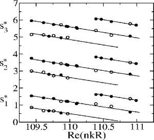
Figure 5: Variation of the optimized bouncing positions ($s_{1}^{*},~{}s_{2}^{*},~{}s_{3}^{*}$). The solid lines denote the present theory with a correction $\mu=0.06$. The circles represent the bouncing positions of triangular quasi-scarred resonance patterns of $n=2$ case; three solid circles with the same $\mbox{Re}(nkR)$ correspond to the main triangular pattern, and three open circles do to the secondary triangular pattern in a quasi-scarred resonance.

We first determine triangles with minimum uncertainty $\alpha$ as a function of $s_{1}$, and then apply the condition of minimum $\beta$ to the triangles. From this process we get the most optimized triangle of ($s_{1}^{*},~{}s_{2}^{*},~{}s_{3}^{*}$) for a fixed $\mbox{Re}(nkR)$. The direct application of this method shows systematic deviation from bouncing positions of resonance patterns. This systematic discrepancy results from the fact that rays inside microcavity have angular distributions and, also the boundary has curvatures, which gives rise to a correction of the Snell’s law. This effect is prominent near the critical angle $\theta_{c}$, studied and known as Goos-Hänchen Go47 and Fresnel Filtering effects Re02 ; Tu02 . We here incorporate these effects by taking effective segment length $l^{*}_{i}=l_{i}+\mu\lambda$. The results are shown in Fig. 5. The solid lines are results of the present theory with $\mu=0.06$ which are in good agreement with the bouncing positions (denoted by circles) of the quasi-scarred resonances. Absence of bouncing positions near $s=2.0$ and $s=4.5$ is consistent with the tentacular structure of the approximate steady probability distribution $P_{s}(s,p)$ in Fig. 2 (a).

In conclusion, we have found that the localized patterns of resonances in a spiral-shaped dielectric microcavity are constructed by the quasi-scar phenomenon which comes from inherent properties of the dielectric microcavity, and that a large fraction of the resonances are quasi-scarred. The results are contrasted with the case of billiard systems in which only scar phenomenon exists, and a small fraction of eigenfunctions are scarred. Even though the system is chaotic, it is possible to extract some information on resonance patterns from the ray dynamical consideration, more precisely, from the steady probability distribution $P_{s}(s,p)$. Since $P_{s}(s,p)$ contains long lasting ray dynamical information, its structure should be related to the high-$Q$ resonances which are likely to appear as lasing modes. From a theoretical viewpoint, just like the semiclassical approach in Hamiltonian systems Cr92 , a semiclassical method in dielectric cavities might be useful to understand resonance positions and degree of scarring or quasi-scarring. Developing semiclassical theory for dielectric cavities seems to be nontrivial. We expect that the results of this Letter will improve physical insight onto resonance patterns in microcavities.

This work is supported by Creative Research Initiatives of the Korean Ministry of Science and Technology. S.-Y. Lee would like to thank S.W. Kim for useful discussion during the Focus Program of APCTP.

References

- (1) E. J. Heller, Phys. Rev. Lett. 53, 1515 (1984).
- (2) O. Bohigas, M. J. Giannoni, and C. Schmit, Phys. Rev. Lett. 52, 1 (1984).
- (3) S. C. Creagh, S.-Y. Lee, and N. D. Whelan, Ann. Phys. 295, 194 (2002); S.-Y. Lee and S. C. Creagh, Ann. Phys. 307, 392 (2003).
- (4) S. Sridhar, Phys. Rev. Lett. 67, 785 (1991); S. Sridhar and E. J. Heller, Phys. Rev. A 46, R1728 (1992).
- (5) T. M. Fromhold, P. B. Wilkinson, F. W. Sheard, L. Eaves, J. Miao, and G. Edwards, Phys. Rev. Lett. 75, 1142 (1995).
- (6) A. Kudrolli, M. C. Abraham, and J. P. Gollub, Phys. Rev. E 63, 026208 (2001).
- (7) S.-B. Lee, J.-H. Lee, J.-S. Chang, H.-J. Moon, S. W. Kim, and K. An, Phys. Rev. Lett. 88, 033903 (2002); T. Harayama, T. Fukushima, P. Davis, P. O. Vaccaro, T. Miyasaka, T. Nishimura, and T. Aida, Phys. Rev. E 67, 015207(R) (2003).
- (8) N. B. Rex, H. E. Tureci, H. G. L. Schwefel, R. K. Chang, and A. D. Stone, Phys. Rev. Lett. 88, 094102 (2002).
- (9) C. Gmachl, F. Capasso, E. E. Narimanov, J. U. Nöckel, A. D. Stone, J. Faist, D. L. Sivco, and A. Y. Cho, Science 280, 1556 (1998).
- (10) C. Gmachl, E. E. Narimanov, F. Capasso, J. N. Ballargeon, and A. Y. Cho, Opt. Lett. 27, 824 (2002).
- (11) Optical Processes in Microcavities, edited by R. K. Chang and A. J. Campillo (World Scientific, Singapore, 1996).
- (12) G. D. Chern, H. E. Tureci, A. D. Stone, R. K. Chang, M. Kneissl, and N. M. Johnson, Appl. Phys. Lett. 83, 1710 (2003).
- (13) J. Hawkes and I. Latimer, Lasers; Theory and Practice (Prentice Hall, 1995).
- (14) J. Schneider, T. Tél, and Z. Neufeld, Phys. Rev. E 66, 066218 (2002); J. Aguirre, and M. A. F. Sanjuán, ibid. 67, 056201 (2003), and references therein.
- (15) J. Wiersig, J. Opt. A: Pure Appl. Opt. 5, 53 (2003).
- (16) Y.-H. Kim, M. Barth, H.-J. Stöckmann, and J. P. Bird, Phys. Rev. B 65, 165317 (2002).
- (17) G. R. Fowles, Introduction to Modern Optics (Holt, Rinehart and Winston, 1975).
- (18) F. Goos and H. Hänchen, Ann. Phys. (Leipzig) 1, 333 (1947); M. Hentschel and H. Schomerus, Phys. Rev. E 65, 045603(R) (2002).
- (19) H. E. Tureci and A. D. Stone, Opt. Lett. 27, 7 (2002).
- (20) M. C. Gutzwiller, J. Math. Phys. 8 1979 (1967); Ozorio de Almeida and Hannay, J. Phys. A: Math. Gen. 20, 5873 (1987); S. C. Creagh and R. G. Littlejohn, ibid. 25, 1643 (1992).