Fractal properties of the diffusion coefficient
in a simple deterministic dynamical system:
a numerical study

Abstract

Using a numerical library for arbitrary precision arithmetic I study the irregular dependence of the diffusion coefficient on the slope of a piecewise linear map defining a dynamical system. I find that the graph of the diffusion coefficient as a function of the slope has the fractal dimension 1, but the convergence to this limit is slowed down by logarithmic corrections. The exponent controlling this correction depends on the slope and is either 1 or 2 depending on existence and properties of a Markov partition.

05.45.Pq, 05.45.Ac, 45.30.+s

1 Introduction

Determining the transport coefficients of many-particle systems is one of the fundamental problems of nonequilibrium statistical physics. This is also a notoriously difficult problem: it turns out that even in a simplified system where a single particle moves in a periodic array of scatterers, the drift and diffusion coefficients are highly irregular, apparently nowhere differentiable functions of control parameters [1, 2, 3, 4] (an example is also shown in Fig. 1 below). Closer inspection of these functions reveals that usually their “irregularities” are not random, but rather form patterns. This has led some researchers to the idea that the graphs of these functions are fractals with nontrivial, perhaps locally varying fractal dimension. This is an interesting concept, since fractal structures are quite commonly found in dynamical systems in various contexts [3, 4].

Until very recently no reliable investigation of fractal properties of transport coefficients was possible because all general methods of calculating transport coefficients in dynamical systems – e.g. the transition matrix technique combined with the escape rate formalism [1, 2, 3, 4, 5, 6], the Green-Kubo formula [1, 3, 4], or the periodic-orbit formalism [3, 7] – eventually lead to complicated and time-consuming numerical calculations. Moreover, usually they are applicable only for some special values of the control parameters. For these reasons none of them could be used to collect a sufficiently large number (counted at least in millions) of very precise data required in fractal analysis. This situation changed when Groeneveld and Klages [8] gave exact formulas for the transport coefficients in a simple one-dimensional dynamical system introduced by Grossmann and Fujisaka [9].

The system investigated by Groeneveld and Klages can be considered as a model of a particle moving in a one-dimensional array of scatterers. The role of the equation of motion is played by a one-dimensional map $M$

$$x_{n+1}=M_{a,b}(x_{n})$$ (1)

where $n$ is a discrete-time variable and the map $M_{a,b}\colon\mathbf{R}\to\mathbf{R}$ is given by a simple linear function

$$M_{a,b}(x)=ax+b,\quad x\in I_{0}^{-}$$ (2)

on the fundamental interval $I_{0}^{-}=[-\textstyle{\frac{1}{2}},\textstyle{\frac{1}{2}})$, with $a>1,b\in\mathbf{R}$ being the control parameters representing the slope and the bias of the map, respectively; the map is then continued periodically onto the real line by a lift of degree one, i.e. by requiring that

$$M_{a,b}(x+1)=M_{a,b}(x)+1,\quad x\in\mathbf{R}.$$ (3)

For $a>1$ the Lyapunov exponent of this system is positive, and so the dynamics defined by $M_{a,b}$ is chaotic. If we choose an arbitrary number $x_{0}$ as the starting point, the resulting sequence $(x_{n})$ will almost always look “random” (the set of points $x_{0}$ generating a regular, periodic or quasi-periodic sequence $(x_{n})$ is of Lebesgue measure 0). For suitably chosen values of $a$ and $b$ the deterministic dynamics defined by the map $M_{a,b}$ is equivalent to a Markov stochastic process of random-walk type: each deterministic trajectory $(x_{n})$ is equivalent to some particular realization of the corresponding random-walk process, and taking the average over all initial states is equivalent to calculating averages over the corresponding Gibbs ensamble. Actually any random-walk Markov process in a one-dimensional periodic system with fixed transition rates can be translated into the language of simple piecewise linear deterministic maps [10]. From this point of view there is no surprise that the process defined by $M_{a,b}$ (or similar maps) is called “deterministic diffusion” and that the two basic transport coefficients, the drift velocity $J$ and diffusion constant $D$, can be defined as

$$J=\lim_{n\to\infty}\frac{\langle x_{n}\rangle}{n},\qquad D=\lim_{n\to\infty}\frac{\langle x_{n}^{2}\rangle-\langle x_{n}\rangle^{2}}{2n}$$ (4)

where $\langle\cdots\rangle$ denotes the average over the uniform ensamble of initial values $x_{0}$.

The graph of the diffusion coefficient $D$ for the map $M_{a,b}$ as a function of the slope $a$ for the bias $b=0$ is shown in Fig. 1. The fractal properties of this highly irregular graph (as well as that of the drift velocity $J$) were recently studied by Klages and Klauß [11]. Using two numerical methods: the box counting and the autocorrelation function methods, they found that the local fractal dimensions of graphs of $J$ and $D$ are well-defined, but highly irregular functions of $a$ and $b$. In other words they found that the graph shown in Fig. 1 cannot be described with a single fractal dimension, but rather by a set of quickly varying local fractal dimensions. Taking this into account they suggested that the local fractal dimensions of graphs of $J$ and $D$ as functions of the slope $a$ with the bias $b$ fixed are fractal themselves. This, in turn, leads to the concept of a “fractal fractal dimension of deterministic transport coefficients” [11].

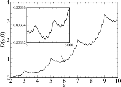
Figure 1: The diffusion coefficient $D$ for the map $M_{a,b}$ as a function of the slope $a$ for the bias $b=0$. The inset depicts a blow-up of a region $6\leq a\leq 6.0001$ (pointed at by the arrow).

Klages and Klauß found the local fractal dimension $\mathcal{D}$ of $J(a,b)$ and $D(a,b)$ to be very close to 1. The autocorrelation function method gave $1.05\lesssim\mathcal{D}\lesssim 1.15$, and the box-counting method gave even lower values $1.02\lesssim\mathcal{D}\lesssim 1.05$. All these values are very close to 1, i.e.  the fractal dimension of a regular, “smooth” curve. This suggests that perhaps $\mathcal{D}=1$ and that the results obtained in the above-mentioned computer simulations reflected extremely slow convergence of $\mathcal{D}$ to its true asymptotic limit of infinitesimally small “boxes”. Such slow convergence is often caused by logarithmic corrections. The main purpose of my paper is thus to try and find such tiny corrections. To accomplish this task I will use a different method of calculating the local fractal dimension of a curve – the so called oscillation method [12] – and I will carry out all calculations with a help of a special high-accuracy numerical library, which will enable me to consider exceptionally small “boxes”. For sake of simplicity I shall restrict the present study to the simplest case of zero bias ($b=0$) where, due to symmetry, the drift velocity $J=0$.

The structure of the paper is as follows. Section 2 briefly describes the method I have used to determine the local fractal dimension. It describes all steps necessary to calculate the diffusion coefficient for the map $M_{a,b}$, a method of calculating the local fractal dimension of a continuous curve (“the oscillation method”), mathematical formulation of the main conjecture about the logarithmic convergence of the fractal dimension to its limiting value, and the numerical aspects of the algorithms used. Section 3 presents the main results. Finally, section 4 is devoted to discussion of results.

2 Method

2.1 Transport coefficient

The explicit formulas [8] for the transport coefficients in the model depend on some auxiliary variables. For each $a>1,b\in\mathbf{R}$, and $\epsilon=\pm$ we define two infinite sequences, $(y_{r}^{\epsilon})$, $r=0,1,\ldots$, and $(n_{r}^{\epsilon})$, $r=1,2,\ldots$, consisting of real and integer numbers, respectively. Their values are uniquely determined by demanding that $y_{0}^{\epsilon}=\frac{\epsilon}{2}$ and that for each $r>0$

$$n_{r}^{\epsilon}+y_{r}^{\epsilon}=ay^{\epsilon}_{r-1}+b,$$ (5)

with additional conditions $n_{r}^{\epsilon}\in\mathbb{Z}$ and $y_{r}^{\epsilon}\in I^{\epsilon}_{0}$, where $I_{0}^{+}\equiv\left(-\textstyle{\frac{1}{2}},\textstyle{\frac{1}{2}}\right]$ and $I_{0}^{-}\equiv\left[-\textstyle{\frac{1}{2}},\textstyle{\frac{1}{2}}\right)$. Next we define “N-numbers”:

$$N_{r}^{\epsilon}=-\frac{\epsilon}{2}+\sum_{s=1}^{r}n_{s}^{\epsilon},$$ (6)

$$N_{k,l}=\frac{1}{k!l!}\sum_{r=0}^{\infty}a^{-r}[(N_{r}^{+})^{k}-(N_{r}^{-})^{k}]r^{l},$$ (7)

where $r,k,l\geq 0$. The basic transport coefficients, $J$ and $D$, can be now expressed ([8], cf [13]) as

$$J=\frac{N_{2,0}}{N_{1,1}},\quad D=\frac{N_{3,0}-N_{2,1}J+N_{1,2}J^{2}}{N_{1,1}}.$$ (8)

2.2 The oscillation method

The fractal dimension $\mathcal{D}$ of a continuous function $f$ defined on an interval $[t_{0},t_{1}]$ can be evaluated through analysis of its Hölder exponents [12] and $\tau$-oscillations [12]. The $\tau$-oscillation of $f$ at $t\in(t_{0},t_{1})$ is defined as

$$\text{osc}_{\tau}(f;t)=\sup_{|t-t^{\prime}|\leq\tau}f(t^{\prime})-\inf_{|t-t^{\prime}|\leq\tau}f(t^{\prime}).$$ (9)

If there exist constants $c>0$ and $0<H\leq 1$ such that for all $\tau$

$$\text{osc}_{\tau}(t)\leq c\tau^{H}$$ (10)

then $f$ is called a Holderian of exponent $H$ at $t$ and its fractal dimension $\mathcal{D}$ at $t$ is related to $H$ through

$$\mathcal{D}\leq 2-H.$$ (11)

Similarly, if there exist constants $c>0$ and $0<H\leq 1$ such that for all $\tau$

$$\text{osc}_{\tau}(t)\geq c\tau^{H}$$ (12)

then $f$ is called an anti-Holderian of exponent $H$ at $t$ and

$$\mathcal{D}\geq 2-H.$$ (13)

2.3 Reformulation of the problem and numerical implementation

We are now ready to formulate our main conjecture: for the map $M_{a,b}$ with $b=0$

$$\frac{\text{osc}_{\tau}(D;a)}{\tau}\approx c(a)\left[-\log(\tau)\right]^{\gamma(a)},\quad\mathrm{as~{}}\tau\to 0,$$ (14)

where the prefactor $c(a)>0$ and the exponent $\gamma(a)\geq 0$. Owing to (9) – (13) this implies that the fractal dimension of the graph of $D$ as a function of the control parameter $a$ is equal 1, but the convergence to this limiting value is logarithmically slow, with the exponent $\gamma(t)$ controlling the convergence rate.

I checked conjecture (14) using equations (5) – (8). Because the consecutive terms of the sequences $n_{s}^{\pm}$ in (6) can be generated extremely efficiently (it took less than a second to generate 20 000 data points used to draw Figure 1), I decided to employ GMP (GNU multiple precision arithmetic library, version 4.1.2) – a library for arbitrary precision arithmetic [14]. Although any calculations performed by such a library must be several orders of magnitude slower that those performed directly, thanks to the GMP I was able to study numerically the limit of $\tau\to 0$ for $\tau$ ranging from $1$ down to at least $10^{-100}$ (the accuracy of typical computers currently available, without using such special-purpose libraries, is limited typically to about $10^{-17}$). Such fine resolution of my calculations will turn out crucial for determining logarithmic corrections predicted by formula (14).

3 Results

In my present study I decided to concentrate on verifying conjecture (14) for the symmetrical case of vanishing bias ($b=0$) and for several selected values of the slope $a$. I decided to examine especially carefully the slopes corresponding to finite Markov partitions. These values are particularly interesting from the theoretical point of view [1, 2, 3]; for example, even though the diffusion coefficient $D$ is always continuous in $a$ [8], the numerator and denominator in (7) can be discontinuous for such (and only such) slopes. One of the reasons why I chose to set $b=0$ is that in this case the slopes corresponding to Markov partitions can be found easily on a computer: they are algebraic numbers generating periodic sequences $n_{k}$ and $y_{k}$. Such values of $a$ will be henceforth referred to as “Markov slopes”.

Figure 2 presents results obtained for two Markov slopes generating strictly periodic sequences (i.e., $y^{\epsilon}_{k+l}=y^{\epsilon}_{k}$ for a period $l>0$ and all $k\geq 0$). The value used in Fig. 2a is $a=3$. This slope generates simple sequences $y^{+}_{k}$ and $y^{-}_{k}$ of period 1. The oscillations of the diffusion coefficient on intervals $(3-\textstyle{\frac{1}{2}}\tau,3+\textstyle{\frac{1}{2}}\tau)$, rescaled by $\tau$, obtained for $\tau=10^{-n},n=1\ldots 100$, are represented in this plot by circles, while the solid line represents a quadratic fit of form $px^{2}+qx+r$ with $p=0.733$, $q=0.57$, and $r=-0.2$. The fit is excellent, which suggests that for this slope the exponent $\gamma$, as defined in eq. (14), is 2. I have obtained similarly good quadratic fits for other integer odd slopes, which also generate simple sequences of period 1 [2].

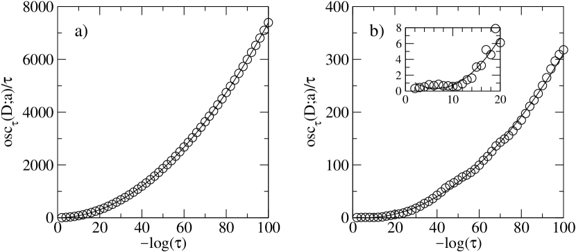
Figure 2: Oscillations of the diffusion coefficient rescaled in accordance with eq. (14) calculated on intervals $(a-\textstyle{\frac{1}{2}}\tau,a+\textstyle{\frac{1}{2}}\tau)$ for $\tau=10^{-n},n=1,\ldots,100$ and for (a) $a=3$ and (b) $a\approx 3.314$. The circles represent results calculated from conjecture (14), and the solid lines are quadratic fits. The inset in graph (b) shows the blow-up of results obtained for $1>\tau\geq 10^{-20}$.

A question arises whether the length of the period has any influence on the limiting value of $\mbox{osc}_{\tau}(\mathcal{D};a)/\tau$. Figure 2b shows the results obtained for the largest root of the polynomial $a^{4}-4a^{3}+2a^{2}+3$, i.e. for $a\approx 3.314$. For this slope the period $l=4$. Just as in the previous example, $\mbox{osc}_{\tau}(\mathcal{D};a)/\tau$ can be approximated by a quadratic, although the fit is not as excellent as for $a=3$. The inset in this figure depicts the blow-up of the data obtained for $1>\tau\geq 10^{-20}$. It shows that for $1>\tau>10^{-10}$ the value of $\mbox{osc}_{\tau}(\mathcal{D};a)/\tau$ fluctuates about a constant value, which might suggest that the exponent $\gamma$ vanishes. This example demonstrates that the “resolution” of calculations used in ref. [11], e.i. $\tau_{\mathrm{min}}\lesssim 10^{-10}$, is insufficient to find the true asymptotic fractal properties of the graph of the diffusion coefficient as a function of the slope $a$.

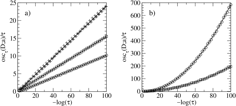
Figure 3: The same as in Fig. 2. (a) $a=4$ (circles), $a\approx 3.3497$ (squares), $a\approx 3.043$ (pluses) with linear fits (solid lines); (b) $a\approx 3.160$ (circles), $a\approx 4.200$ (squares) with quadratic fits (solid lines). See text for details.

All other Markov slopes generate sequences $n_{k}^{\epsilon}$ and $y_{k}^{\epsilon}$ with the period starting at a term $m>0$. There are two cases: either all terms of $y_{k}^{+}$ are different from all the terms of $y_{k}^{-}$ or the two sequences have the same period sequence. Let’s start from the latter case. Three examples of results obtained for Markov slopes of this type are shown in Figure 3a. The data depicted in this graph were calculated for $a=4$ (circles), for the largest root of $a^{4}-4a^{3}+2a^{2}+2$, i.e. for $a\approx 3.3497$ (squares), and for the largest root of $a^{5}-4a^{4}+2a^{3}+3a^{2}-2a+4$, i.e. for $a\approx 3.043$ (pluses). For the first two of the above slopes all the terms of the sequences $y_{k}^{\epsilon}$ eventually vanish. In the case of $a=4$ this happens for $k\geq 1$, and for $a\approx 3.3497$ the terms of $y^{\epsilon}_{k}$ vanish for $k\geq 4$. As for the third example, $a\approx 3.043$, the period starts at $k=2$ and has the length 6. Specifically, the first five terms of $y_{k}^{+}$ are (to 3 S.F.) $1/2$, $-0.478$, $-0.456$, $-0.387$, $-0.179$, and for $k\geq 5$ the terms satisfy $y_{k}^{+}=-y_{k-3}^{+}=y_{k-3}^{-}$. As we can see, in all these cases $\mbox{osc}_{\tau}(\mathcal{D};a)/\tau$ diverges linearly with $\log(\tau^{-1})$, suggesting that conjecture (14) is satisfied with the exponent $\gamma=1$.

The results obtained for the last category of Markov slopes, i.e. slopes generating two disjoint periodic sequences $y_{k}^{+}$ and $y_{k}^{-}$, are shown in Fig. 3b. The two data sets were collected for the largest root of $a^{5}-4a^{4}+2a^{3}+a^{2}+4a-2$, i.e. for $a\approx 3.16$ (circles) and for the largest root of $a^{5}-4a^{4}-4a^{2}+a+4$, i.e. for $a\approx 4.20$ (squares). The first of these slopes, $a\approx 3.16$, generates a sequence with a period of length 3 starting at $y_{2}^{+}$, while $a\approx 4.20$ generates a sequence of period length 4 starting at $y_{1}^{+}$. As we can see, for these Markov slopes $\mbox{osc}_{\tau}(\mathcal{D};a)/\tau$ can be very well approximated by a quadratic function of $\log(\tau^{-1})$. This suggests that in this case conjecture (14) is satisfied with the exponent $\gamma=2$.

Figure 4 presents results for two slopes $a$ which do not correspond to a Markov partition. These are $a=\pi\approx 3.14$ (left panel) and $a=9/2$ (right panel). The results turned out to be “noisy” and I had to increase the resolution down to $\tau_{\mathrm{min}}=10^{-300}$. As can be seen, in both cases $\mbox{osc}_{\tau}(\mathcal{D};a)/\tau$ has a clear trend linear in $\log(\tau^{-1})$. However, this limiting behaviour is disturbed by very large fluctuations. Actually, for $a=\pi$ these fluctuations are so large that my numerical results cannot rule out the possibility that in this case the limit $\lim_{\tau\to 0}\mbox{osc}_{\tau}(\mathcal{D};a)/\tau$ does not exist.

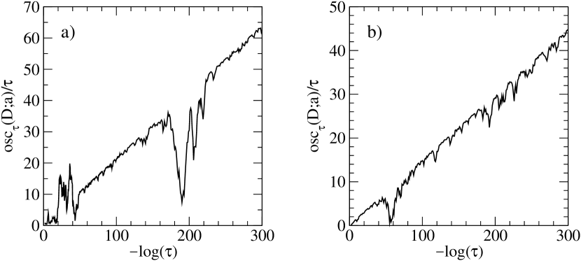
Figure 4: The same as in Fig. 2 for two slopes $a$ that do not correspond to finite Markov partitions: (a) $a=\pi\approx 3.14$ and (b) $a=4.5$.

4 Conclusions

In my study I proposed and verified numerically a hypothesis that the local fractal dimension of the graph of the diffusion coefficient of the piecewise linear map $M_{a,b}$ as a function of the slope $a$ is $\mathcal{D}=1$ and that the convergence to this limit is slowed down by logarithmic corrections described by eq. (14). This contradicts the earlier findings of Klages and Klauß [11] that this graph is a fractal with a locally varying fractal dimension $\mathcal{D}(a)>1$ which, when plotted as a function of the slope, forms a fractal itself.

I found that the exponent $\gamma$, which controls the logarithmic correction, is actually a function of the slope $a$. Interestingly, $\gamma$ appears to be a discontinuous function that can take only one of two values: 1 or 2. The value of 1 corresponds to Markov slopes that generate two disjoint sequences $y_{k}^{+}$ and $y_{k}^{-}$, and the value of $\gamma=2$ corresponds to Markov slopes that generate periodic sequences $y_{k}^{+}$ and $y_{k}^{-}$ with the same period terms. The case of slopes that do not generate Markov partitions is not clear – apparently $\gamma=1$, but this statement cannot be verified numerically because of very large fluctuations making the convergence extremely slow. Note that my findings imply that both of the sets $\{a\colon\gamma(a)=1\}$ and $\{a\colon\gamma(a)=2\}$ are dense, and hence that $\gamma(a)$ is nowhere continuous.

Any numerical study is naturally restricted to investigation of several particular cases. It cannot be ruled out that I have overlooked some categories of slopes $a$ for which the local fractal dimension of the graph of the diffusion coefficient behaves in a way not predicted in this study. Numerical investigation of the logarithmic correction to the asymptotic limit is here a particularly delicate problem, as apparently $\gamma$ is a nowhere continuous function of the slope. Only through an analytical approach could this problem be solved conclusively. Such a study will be published elsewhere.

References

- [1] R. Klages, Deterministic Diffusion in One-Dimensional Chaotic Dynamical Systems, Wissenschaft und Technik Verlag, Berlin 1996.
- [2] R. Klages and J. R. Dorfman, Phys. Rev. E 59, 5361 (1999).
- [3] J. R. Dorfman, An Introduction to Chaos in Nonequilibrium Statistical Mechanics, Cambridge University Press, Cambridge 1999.
- [4] R. Klages, Microscopic Chaos, Fractals, and Transport in Nonequilibrium Steady States, (habilitation thesis) TU Dresden, submitted 2003.
- [5] P. Gaspard and G. Nicolis, Phys. Rev. Lett. 65, 1693 (1990).
- [6] P. Gaspard J. Stat. Phys. 68, 673 (1992).
- [7] P. Cvitanović, R. Artuso, R. Mainieri, G. Tanner, and G. Vattay, Chaos: classical and quantum, ChaosBook.org, Niels Bohr Insitute, Copenhagen 2003.
- [8] J. Groeneveld and R. Klages, J. Stat. Phys. 109, 821 (2002).
- [9] S. Grossmann and H. Fujisaka, Phys. Rev. A 26, 1779 (1982).
- [10] I. Claes and C. Van den Broeck, J. Stat. Phys. 70, 1215 (1993).
- [11] R. Klages and T. Klauß, J. Phys. A: Math. Gen. 36, 5747 (2003).
- [12] C. Tricot, Curves and Fractal Dimension, Springer, Berlin 1995.
- [13] Z. Koza, J. Phys. A: Math. Gen. 32, 7637 (1999).
- [14] see: http://www.swox.com/gmp.