Comment on “Shadowability of Statistical Averages in Chaotic Systems”

Lai et al. Lai:2002 investigate systems with a stable periodic orbit and a coexisting chaotic saddle. They claim that, by adding white Gaussian noise (GN), averages change with an algebraic scaling law above a certain noise threshold and argue that this leads to a breakdown of shadowability of averages. Here, we show that (i) shadowability is not well defined and even if it were, no breakdown occurs. We clarify misconceptions on (ii) thresholds for GN. We further point out (iii) misconceptions on the effect of noise on averages. Finally, we show that (iv) the lack of a proper threshold can lead to any (meaningless) scaling exponent.
(i) Shadowing deals with macroscopic error propagation of noise bounded by a small value (e.g. computer accuracy of $10^{-16}$), comparing a noisy and a ‘true’ trajectory Grebogi:1990 . Since the authors use GN, one cannot properly speak of shadowing. However, even for bounded noise, their claims are still doubtful. In a recent work, the error of an average was found to be amplified by a factor of up to $10^{12}$, although the trajectory never exits the attractor Sauer:2002 . This renders a reliable computation truly unfeasible. In Lai:2002 , though, the effect on the averages is only of the same order as the variation of the noise level $D$. Furthermore, the averages in Figs. 1a and 2a in Lai:2002 do change even less below $D=10^{-2.5}$. Therefore, shadowability is not compromised at all.
(ii) The authors of Lai:2002 mention a threshold for GN above which the periodic orbit and the chaotic saddle would become connected. Yet, such a threshold does not exist, since the mean first exit time $\langle\tau\rangle$ is given by Kramers’ law $\langle\tau\rangle\sim\exp(\frac{\Delta U}{D})$, where $D$ is the noise variance and $\Delta U$ is either the potential Kramers:1940 or, for nonequilibrium and chaotic systems, the quasipotential difference Graham:1984 . Thus, $\langle\tau\rangle$ varies with $D$, yielding a different average for every noise level.
(iii) Generally, averages depend on the noise for all noise levels, implying that no threshold can exist, even with only one metastable state. For the linear map $x_{n+1}=ax_{n}+b+\xi_{n}$ with a fixed point $x_{\star}=\frac{b}{1-a}$ and white GN one gets $\langle x^{2}\rangle=x_{\star}^{2}+\frac{1}{1-a^{2}}\,D$. This is pictured in Fig. 1a, fitting perfectly the data. Although the average appears to be constant for low noise, it depends, in fact, on the noise for all $D$. The same applies also to nonlinear systems (cf. fit in Fig. 1b) and bounded noise.
(iv) Because the value of the threshold is arbitrary, any scaling can be achieved, just by tuning $D_{c}$, as fittings of the form of Eq. (1) of Lai:2002 are very sensitive to the value of $D_{c}$. To verify this, we show in Fig. 1b the logistic map $x_{n+1}=ax_{n}(1-x_{n})+D\,\xi_{n}$ with $\langle\xi_{n},\xi_{m}\rangle=\delta_{nm}$ as in Lai:2002 . The putative threshold of $D_{c}=10^{-5}$ is marked by an arrow. The graph is evidently not constant there. With $D_{c}\approx 7\cdot 10^{-6}$ (first arrow), a scaling $\Delta G\sim(D-D_{c})^{\alpha}$ results, with $\Delta G$ of Lai:2002 . This yields $\alpha\approx 2.1$ (Fig. 1c), in clear contrast to $\alpha\approx 1$ reported in Lai:2002 . Therefore, no reliable (i. e. any) exponent can be obtained, since $D_{c}$ is not well defined from the outset.

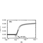
Figure 1: (a) $\langle x^{2}\rangle$ for the linear map vs. $D$ with $a=0.7$ and $b=0.75$ (circles) and analytical fit $\langle x^{2}\rangle=x_{\star}^{2}+\frac{1}{1-a^{2}}\,D$ (full line). (b) $\langle\sin\,x\rangle$ for the logistic map with $a=3.8008$ and a polynomial fit for $D\,\leq\,1.4\cdot 10^{-5}$ (full line) (c) Scaling $\Delta G\sim(D-D_{c})^{\alpha}$ with $D_{c}\approx 7\cdot 10^{-6}$ (circles) and least squares fit (full line). All averages are for $10^{8}$ iterations.

As to the reply, the authors claim to have “a theoretical justification for the existence of a threshold” through $D_{c}=\sqrt{{\Delta\Phi}/\ln\chi^{-1}}$, with ${\Delta\Phi}$ the quasipotential (see (ii)) and $\chi$ the probability resolution. Contrary to Ref. [5] of the reply, where $\chi$ drops out since only proportionalities under parameter variation are considered, $D_{c}$ in Lai:2002 depends for fixed parameters on $\chi$ and hence $\alpha$ is not uniquely defined. Applied to (iv) with $D_{c}=10^{-5}$ of Lai:2002 and ${\Delta\Phi}\approx 7.8\cdot 10^{-10}$ (not shown) yields $\chi=0.0004$. But a finer resolution $\chi=10^{-7}$ gives $D_{c}=7\cdot 10^{-6}$, with $\alpha\approx 2.1$ (cf. (iv)), whereas $\chi=10^{-2}$ results in $D_{c}=1.3\cdot 10^{-5}$ and $\alpha\approx 0.21$ (not shown). Again, this invalidates any proper scaling.


Suso Kraut
Instituto de Física, Universidade de São Paulo
Caixa Postal 66318, 05315-970 São Paulo, Brazil

References

- (1) Y. C. Lai et al., Phys. Rev. Lett. 89, 184101 (2002).
- (2) C. Grebogi et al., Phys. Rev. Lett. 65, 1527 (1990).
- (3) T. D. Sauer, Phys. Rev. E 65, 036220 (2002).
- (4) H. A. Kramers, Physica 7, 284 (1940).
- (5) R. Graham and T. Tél, Phys. Rev. Lett. 52, 9 (1984); R. Graham, A. Hamm, and T. Tél, ibid 66, 3089 (1991).