Resonant and Non-Resonant Modulated Amplitude Waves for Binary Bose-Einstein Condensates in Optical Lattices

Abstract

We consider a system of two Gross-Pitaevskii (GP) equations, in the presence of an optical-lattice (OL) potential, coupled by both nonlinear and linear terms. This system describes a Bose-Einstein condensate (BEC) composed of two different spin states of the same atomic species, which interact linearly through a resonant electromagnetic field. In the absence of the OL, we find plane-wave solutions and examine their stability. In the presence of the OL, we derive a system of amplitude equations for spatially modulated states which are coupled to the periodic potential through the lowest-order subharmonic resonance. We determine this averaged system’s equilibria, which represent spatially periodic solutions, and subsequently examine the stability of the corresponding solutions with direct simulations of the coupled GP equations. We find that symmetric (equal-amplitude) and asymmetric (unequal-amplitude) dual-mode resonant states are, respectively, stable and unstable. The unstable states generate periodic oscillations between the two condensate components, which is possible only because of the linear coupling between them. We also find four-mode states, but they are always unstable. Finally, we briefly consider ternary (three-component) condensates.

PACS: 05.45.-a, 03.75.Lm, 05.30.Jp, 05.45.Ac

I Introduction

At sufficiently low temperatures, particles in a dilute boson gas condense in the ground state, forming a Bose-Einstein condensate (BEC). This was first observed experimentally in 1995 in Na and Rb vapors[37, 16, 26, 12].

In the mean-field approximation, a dilute BEC is described by the nonlinear Schrödinger (NLS) equation with an external potential, which is also called the Gross-Pitaevskii (GP) equation. In particular, BECs may be considered in the quasi-one-dimensional (quasi-1D) regime, with the transverse dimensions of the condensate on the order of its mean healing length $\chi$ (given by $\chi^{2}=(8\pi n|a|)^{-1}$) and a much larger longitudinal dimension [9, 10, 8, 16]. The length $\chi$ is determined by the mean atomic density $n$ and the two-body $s$-wave scattering length $a$, where the interactions between atoms are repulsive if $a>0$ and attractive if $a<0$ [37, 16, 27, 4].

The quasi-1D regime, which corresponds to “cigar-shaped” BECs, is described by the 1D limit of the 3D mean-field theory (rather than by a 1D mean-field theory proper, which would only be appropriate for extremely small transverse dimensions of order $\sim a$) [9, 8, 10, 45, 6]. In this situation, the condensate wave function $\psi(x,t)$ obeys the effective 1D GP equation,

$\displaystyle i\hbar\psi_{t}=-\frac{\hbar^{2}}{2m}\psi_{xx}+g|\psi|^{2}\psi+V(x)\psi,$

where $m$ is the atomic mass, $V(x)$ is an external potential, $g=[4\pi\hbar^{2}a/m][1+O(\eta^{2})]$, and $\eta=\sqrt{n|a|^{3}}$ is the dilute-gas parameter[16, 27, 4, 29]. Experimentally relevant potentials $V(x)$ include harmonic traps and periodic potentials (created as optical lattices, which are denoted OLs and arise as interference patterns produced by coherent counterpropagating laser beams illuminating the condensate). In the presence of both potentials, $V(x)=V_{0}\cos\left[2\kappa(x-x_{0})\right]+V_{1}x^{2}/2$, where $x_{0}$ is the offset of the periodic potential relative to the center of the the parabolic trap. When $\left(2\pi/\kappa\right)^{2}V_{1}\ll V_{0}$, the potential is dominated by its periodic component over many periods [17, 14, 11]; for example, when $V_{0}/V_{1}=500$ and $\kappa=10$, the parabolic component in $V(x)$ is negligible for the 10 periods closest to the trap’s center. In this work, we set $V_{1}=0$ and focus entirely on OL potentials. This assumption is motivated by numerous recent experimental studies of BECs in OLs [22, 3] and is widely adopted in theoretical studies [9, 8, 10, 7, 15, 14, 17, 34, 2, 48, 38, 39, 35, 50, 31, 30].

Multiple-component BECs, which constitute the subject of this work, have been considered in a number of theoretical works [24, 41, 40, 20, 13, 47, 18]. Mixtures of two different species (such as ⁸⁵Rb and ⁸⁷Rb) are described by nonlinearly coupled GP equations:

$$i\hbar\frac{\partial\psi_{1}}{\partial t} =-\frac{\hbar^{2}}{2m_{1}}\nabla^{2}\psi_{1}+g_{1}|\psi_{1}|^{2}\psi_{1}+V(x)\psi_{1}+h|\psi_{2}|^{2}\psi_{1},$$ (1)

$$i\hbar\frac{\partial\psi_{2}}{\partial t} =-\frac{\hbar^{2}}{2m_{2}}\nabla^{2}\psi_{2}+g_{2}|\psi_{2}|^{2}\psi_{2}+V(x)\psi_{2}+h|\psi_{1}|^{2}\psi_{2},$$ (2)

where $m_{1,2}$ are the atomic masses of the species, $g_{j}\equiv 4\pi\hbar^{2}a_{j}/m_{j}$ corresponds to the self-scattering length $a_{j}$, and

$$h\equiv g_{12}=2\pi\hbar^{2}a_{12}\left(m_{1}+m_{2}\right)/\left(m_{1}m_{2}\right)$$ (3)

depends on the cross-scattering length $a_{12}$ [41]. There are numerous subcases of Eqs. (2) to consider, as various combinations of signs for the scattering coefficients $g_{1}$, $g_{2}$, and $h$ may occur. It is important to note, however, that if $g_{1,2}$ are positive (repulsion between the atoms), then $h$ is normally positive as well. However, if $g_{1,2}$ are negative (corresponding to the less typical case of attraction between atoms belonging to a single species), then $h$ [see Eq. (3)] may be either positive or negative.

The system (2) resembles a well-known model describing the nonlinear self-phase-modulation (SPM) and cross-phase-modulation (XPM) interactions of light waves with different polarizations or carried by different wavelengths in nonlinear optics [1]. In the case of optical fibers, the evolution variable is the propagation distance $z$ (rather than time), and the role of $x$ is played by the reduced temporal variable $\tau$ [1]. In optical models, however, the choice of the nonlinear coefficients is limited to the combinations $g_{1}=g_{2}=3h/2$ for orthogonal linear polarizations in a birefringent fiber and $g_{1}=g_{2}=h/2$ for circular polarizations or different carrier wavelengths. In fact, the latter case is quite important in the application to two-component BECs as well, as it occurs if one assumes that the collision lengths for interactions between all the atoms are the same.

Another physically interesting feature, which we include in the model to be considered below, is linear coupling between the two wave functions. This occurs in a mixture of two different spin states of the same isotope, which arises through a resonant microwave field that induces transitions between the states[5, 46]. Condensates containing two different spin states of ⁸⁷Rb have been created experimentally via sympathetic cooling [36]. In this situation, the normalized coupled GP equations take the form

$$i\frac{\partial\psi_{1}}{\partial t} =-\nabla^{2}\psi_{1}+g|\psi_{1}|^{2}\psi_{1}+V(x)\psi_{1}+h|\psi_{2}|^{2}\psi_{1}+\alpha\psi_{2},$$ (4)

$$i\frac{\partial\psi_{2}}{\partial t} =-\nabla^{2}\psi_{2}+g|\psi_{2}|^{2}\psi_{2}+V(x)\psi_{2}+h|\psi_{1}|^{2}\psi_{2}+\alpha\psi_{1},$$ (5)

where the self- and cross-scattering coefficients are ${g_{1}=g_{2}\equiv g}$ and $h$, and the linear coupling coefficient is $\alpha$, which can always be made positive without loss of generality.

Experimental studies of mixtures of two interconvertible condensates (with positive scattering lengths) loaded in an OL have not yet been reported. However, all the necessary experimental ingredients for such a work are currently available. Moreover, in a very recent paper [28], an experimental procedure, based on Ramsey spectroscopy and adjusted exactly for such a system, was elaborated. Experiments in this setting would be quite interesting, as they would allow the study of the direct interplay between two crucially important physical factors used as tools in the current experimental work—namely, the OL potential and inter-conversion between two different spin states in the BEC, controlled by the resonant field. Furthermore, there are now recent experimental results with linearly coupled BECs [23]. The use of an optical potential in the latter setting is a rather straightforward extension.

The model combining nonlinear XPM and linear couplings, as in Eqs. (5), occurs in fiber optics as well. In that case, the linear coupling is generated by a twist applied to the fiber in the case of two linear polarizations, and by an elliptic deformation of the fiber’s core in the case of circular polarizations (see, for example, [32]). However, linear coupling is impossible in the case of two different wavelengths. Another optical model, with only linear coupling between two modes, applies to dual-core nonlinear fibers, as discussed in [33] (and references therein). In the context of BECs, it may correspond to a special case in which the cross-scattering length is made (very close to) zero using a Feshbach resonance [25].

In this work, we aim to investigate modulated-wave states in the binary BEC described by Eqs. (5), which include both nonlinear and linear couplings and an OL potential. We stress that the interplay between the microwave-induced linear coupling in the binary model and the OL-induced periodic potential has never before been considered. As both features represent important laboratory tools, the results reported here suggest possibilities for new experiments. The model we study predicts new dynamical effects, such as oscillations of matter between the linearly-coupled components trapped in the potential wells of the OL.

In our study, we begin by examining plane-wave solutions with $V(x)\equiv 0$. When $V(x)\neq 0$, we apply a standing-wave ansatz to Eq. (5), which leads to a system of coupled parametrically forced Duffing equations describing the spatial evolution of the fields. Using the method of averaging [44, 42], we study periodic solutions of the latter system (called “modulated amplitude waves”and denoted MAWs). The stability of MAWs (and the ensuing dynamics, in the case of instability) is then tested by numerically simulating the underlying system of coupled GP equations. This approach, though simpler than the more “rigorous” computation of linear stability eigenvalues for infinitesimal perturbations, provides a more realistic emulation of physical experiments. Note additionally that although our stability results will be illustrated by a few selected examples, we have checked—by exploring different parameter regions—that these examples represent the MAW stability features rather generally.

The MAW solutions are especially interesting when the system exhibits a spatial resonance. In this work, we consider both non-resonant solutions and solutions featuring a subharmonic resonance of the $2\!:\!1\!:\!1$ form. The latter situation has been studied in the context of period-doubling in single-component BECs in an OL potential [30, 38, 39], but—to the best of our knowledge—spatial-resonance states in models of composite BECs have not been considered previously.

An alternative (but less general) approach to the study of binary BECs with linear coupling, loaded into an OL, would be to seek exact elliptic-function solutions to Eqs. (5) for the case of elliptic-function potentials, $V(x)=-V_{0}{\rm sn}^{2}(\kappa x,k)$, as has been done earlier in the two-component model without linear coupling [18]. In that work, stable standing-wave solutions were found under the assumption that the interaction matrix is positive definite. This occurs, for instance, when all the interactions are repulsive, although small negative cross-interactions are compatible with this condition as well.

The rest of this paper is structured as follows: In section II, we derive plane-wave solutions and analyze their stability. In section III, we introduce modulated amplitude waves, and in section IV, we derive and solve averaged equations that describe them in both non-resonant and resonant situations. We corroborate our results and test the stability of the MAWs using numerical simulations. In section V, we briefly examine a more general model of a ternary (three-component) BEC with linear couplings. Finally, we summarize our results in section VI.

II Plane-Wave Solutions

In the absence of the external potential ($V=0$), we find plane-wave solutions of the form

$$\psi_{j}=R_{j}\exp\left[i(k_{j}x-\mu_{j}t)\right]\,,\quad j=1,2\,.$$ (6)

For the linearly coupled GP equation (5), it is necessary that $k_{1}=k_{2}\equiv k$ and $\mu_{1}=\mu_{2}\equiv\mu$. Without linear coupling, [as in Eqs. (2)], one may seek a broader class of solutions with independent frequencies (which correspond to chemical potentials in the physical context of BECs). It is important to note that the results obtained in the study of optical models suggest that the addition of linear coupling terms to a system of coupled NLS equations drastically alters the dynamical behavior [32]. In this section, we study the model without the OL, which will be included in subsequent sections.

Inserting Eq. (6) into Eqs. (5) yields

$$\mu R_{1} =k^{2}R_{1}+gR_{1}^{3}+hR_{1}R_{2}^{2}+\alpha R_{2}\,,$$ (7)

$$\mu R_{2} =k^{2}R_{2}+gR_{2}^{3}+hR_{1}^{2}R_{2}+\alpha R_{1}\,,$$ (8)

which implies that

$\displaystyle[(g-h)R_{1}R_{2}-\alpha][R_{1}^{2}-R_{2}^{2}]=0\,.$

One of the following two relations must then be satisfied:

$$R_{1}=\pm R_{2}\,;$$ (9)

$$R_{1}R_{2}=\frac{\alpha}{g-h}\,.$$ (10)

With Eq. (9), a nonzero solution satisfies $R_{2}=\pm\sqrt{\left(k^{2}+\mu\mp\alpha\right)/\left(g+h\right)}$. It exists when $g+h>0$, provided $k^{2}+\mu\mp\alpha>0$, and when $g+h<0$, if $k^{2}+\mu\mp\alpha<0$. When $g=-h$, one obtains solutions of the form $\left(R_{1},R_{2}\right)=\left(\pm R,R\right)$ with arbitrary $R$ and $k^{2}=\mu\mp\alpha$.

From Eq. (10), one finds that

$$R_{2}^{2}=\frac{\mu-k^{2}}{2g}\pm\frac{1}{2}\sqrt{\left(\frac{\mu-k^{2}}{g}\right)^{2}-\frac{4\alpha^{2}}{(g-h)^{2}}}\,,$$ (11)

under the restriction that this expression must be positive. When $\alpha\neq 0$, the term inside the square root is smaller in magnitude than the one outside, so solutions of this type exist as long as $\left(\mu-k^{2}\right)g\geq 0$ and the argument of the square root in (11) is non-negative. Hence, for repulsive and attractive BECs, respectively, the first condition implies, $\mu>k^{2}$ and $\mu<k^{2}$. When $h=0$, Eq. (11) takes the form

$\displaystyle R_{2}^{2}=\left(2g\right)^{-1}\left(\mu-k^{2}\pm\sqrt{(\mu-k^{2})^{2}-4\alpha^{2}}\right)\,.$

For both $h=0$ and $h=2g$, the condition on the argument of the square root implies that to obtain real solutions, it is necessary to impose the condition $|\mu-k^{2}|~{}\geq 2\alpha$.

To examine the stability of the plane waves, we substitute

$\displaystyle\psi_{j}(x,t)=\phi_{j}(x,t)[1+\epsilon_{j}(x,t)]\,,\quad|\epsilon_{j}|^{2}\ll 1\,,$

into Eqs. (5). This yields coupled linearized equations for $\epsilon_{1}(x,t)$ and $\epsilon_{2}(x,t)$. Assuming that $\epsilon_{j}$ is periodic in $x$, it can be expanded in a Fourier series,

$\displaystyle\epsilon_{j}(x,t)=\sum_{n=-\infty}^{\infty}\hat{\epsilon}_{jn}(t)\exp(i\nu_{n}x)\,,$

where the $n$th mode has wavenumber $\nu_{n}$. The perturbation growth rates that determine the stability of the $n$th mode are then given by

$$\lambda_{n}=-2ik\nu_{n}\pm\nu_{n}\sqrt{-\nu_{n}^{2}-g(|R_{1}|^{2}+|R_{2}|^{2})\pm\sqrt{g^{2}(|R_{1}|^{2}-|R_{2}|^{2})^{2}+4h^{2}|R_{1}|^{2}|R_{2}|^{2}}}\,,$$ (12)

where the two sign combinations $\pm$ are independent (so there are four distinct eigenvalues). Instability occurs when the expression under the square root in Eq. (12) has a positive real part, causing the side-band modes $k+\nu_{n}$, $k-\nu_{n}$ of the perturbed solution to grow exponentially. In single-component condensates, this can occur only for $g<0$ [49].

Eigenvalues whose interior square root in Eq. (12) has a $+$ sign will produce the instability before ones with a $-$ sign, so we only need to check the former case. For example, if $h=2g$, the instability occurs if

$$\nu_{n}^{2}+g\left(|R_{1}|^{2}+|R_{2}|^{2}-\sqrt{|R_{1}|^{4}+14|R_{1}^{2}R_{2}^{2}|+|R_{2}|^{2}}\right)<0.$$ (13)

Stability conditions for the plane-wave solutions to Eqs. (5) with $V=0$ can be obtained for all the possible sign combinations of $g$ and $h$. We do not display them here, as they are rather cumbersome to write (although straightforward to compute).

III Modulated Amplitude Waves

We now generalize the above analysis to consider the two-component GP system in the presence of an OL potential. Toward this aim, we introduce solutions to Eqs. (5) that describe coherent structures of the form

$$\psi_{j}(x,t)=R_{j}(x)\exp\left[i(\theta(x)-\mu t)\right]\,,\quad j=1,2\,.$$ (14)

Inserting Eq. (14) into Eqs. (5) and equating real and imaginary parts of the resulting equations yields

$$\mu R_{1} =-R_{1}^{\prime\prime}+R_{1}\left(\theta^{\prime}\right)^{2}{}+gR_{1}^{3}+V(x)R_{1}+hR_{2}^{2}R_{1}+\alpha R_{2}\,,$$ (15)

$$\mu R_{2} =-R_{2}^{\prime\prime}+R_{2}\left(\theta^{\prime}\right)^{2}+gR_{2}^{3}+V(x)R_{2}+hR_{1}^{2}R_{2}+\alpha R_{1}\,,$$ (16)

$$0 =R_{1}\theta^{\prime\prime}+R_{1}^{\prime}\theta^{\prime},$$ (17)

$$0 =R_{2}\theta^{\prime\prime}+R_{2}^{\prime}\theta^{\prime},$$ (18)

where the prime stands for $d/dx$. Equations (18) imply that

$$\theta(x)=c_{1}\int\frac{dx^{\prime}}{R_{1}^{2}(x^{\prime})}=c_{2}\int\frac{dx^{\prime}}{R_{2}^{2}(x^{\prime})}\,,$$ (19)

with arbitrary integration constants $c_{1}$ and $c_{2}$, so $R_{1}(x)=bR_{2}(x)$ for some constant $b$ unless $c_{1}=c_{2}=0$. In other words, $R_{1}(x)$ and $R_{2}(x)$ are different in this context only when one considers solutions with null “angular momenta.”  In the latter situation, Eqs. (16) assume the form

$$R_{1}^{\prime} =S_{1}\,,$$ (20)

$$S_{1}^{\prime} =-\mu R_{1}+gR_{1}^{3}+hR_{1}R_{2}^{2}+\alpha R_{2}+V(x)R_{1}\,,$$ (21)

$$R_{2}^{\prime} =S_{2}\,,$$ (22)

$$S_{2}^{\prime} =-\mu R_{2}+gR_{2}^{3}+hR_{1}^{2}R_{2}+\alpha R_{1}+V(x)R_{2}\,.$$ (23)

When the potential $V(x)$ is sinusoidal, Eqs. (23) are (linearly and nonlinearly) coupled cubic Mathieu equations.

IV Averaged Equations and Spatial Subharmonic Resonances

To achieve some analytical understanding of the spatial resonances in linearly coupled BECs, we average equations (23) in the physically relevant case of the OL potential,

$$V(x)=V_{0}\cos(2\kappa x)\,.$$ (24)

Defining $V_{0}\equiv-\epsilon\tilde{V}_{0}$, $g\equiv\epsilon\tilde{g}$, $h\equiv\epsilon\tilde{h}$, and $\alpha\equiv\epsilon\tilde{\alpha}$, Eqs. (23) may be written

$$R_{1}^{\prime\prime}+\mu R_{1} =-\epsilon\tilde{V}_{0}R_{1}\cos(2\kappa x)+\epsilon\tilde{g}R_{1}^{3}+\epsilon\tilde{h}R_{1}R_{2}^{2}+\epsilon\tilde{\alpha}R_{2}\,,$$ (25)

$$R_{2}^{\prime\prime}+\mu R_{2} =-\epsilon\tilde{V}_{0}R_{2}\cos(2\kappa x)+\epsilon\tilde{g}R_{2}^{3}+\epsilon\tilde{h}R_{1}^{2}R_{2}+\epsilon\tilde{\alpha}R_{1}\,.$$ (26)

Assuming $\mu>0$, we insert the ansatz

$$R_{j}(x) =A_{j}(x)\cos\left(\sqrt{\mu}x\right)+B_{j}(x)\sin\left(\sqrt{\mu}x\right)\,,$$ (27)

$$R_{j}^{\prime}(x) =-\sqrt{\mu}A_{j}(x)\sin\left(\sqrt{\mu}x\right)+\sqrt{\mu}B_{j}(x)\cos\left(\sqrt{\mu}x\right)$$ (28)

(with $j=1,2$) into Eqs. (26). Differentiating the first equation of (28) and comparing it with the second yields a consistency condition,

$\displaystyle A_{j}^{\prime}\cos(\sqrt{\mu}x)+B_{j}^{\prime}\sin(\sqrt{\mu}x)=0\,,\quad j=1,2\,,$

that must be satisfied for this procedure to be valid. Inserting these equations into Eqs. (26) yields a set of coupled differential equations for $A_{j}$ and $B_{j}$, whose right-hand sides are expanded as truncated Fourier series to isolate contributions from different harmonics [44, 42]. The leading contribution in these equations is of $O(\epsilon)$, so the equations assume a general form

$$A_{j}^{\prime} =\epsilon F_{A_{j}}(A_{1},A_{2},B_{1},B_{2},x)+O(\epsilon^{2})\,,$$ (29)

$$B_{j}^{\prime} =\epsilon F_{B_{j}}(A_{1},A_{2},B_{1},B_{2},x)+O(\epsilon^{2})\,.$$ (30)

When $\epsilon=0$, Eqs. (26) decompose into two uncoupled harmonic oscillators. We have computed the exact functions $F_{A_{j}}$ and $F_{B_{j}}$ in Eqs. (30) and provide them in the Appendix.

Our objective is to isolate the parts of the functions $A_{j}(x)$ and $B_{j}(x)$ that vary slowly in comparison with the fast oscillations of $\cos(\sqrt{\mu}x)$ and $\sin(\sqrt{\mu}x)$ and to derive averaged equations governing their slow evolution. To commence averaging, we decompose $A_{j}$ and $B_{j}$ into the sum of slowly varying parts and small rapidly oscillating ones (which are written as power-series expansions in $\epsilon$):

$$A_{j} =\bar{A}_{j}+\epsilon W_{A_{j}}(\bar{A}_{1},\bar{A}_{2},\bar{B}_{1},\bar{B}_{2},x)+O(\epsilon^{2}),$$ (31)

$$B_{j} =\bar{B}_{j}+\epsilon W_{B_{j}}(\bar{A}_{1},\bar{A}_{2},\bar{B}_{1},\bar{B}_{2},x)+O(\epsilon^{2})\,.$$ (32)

Here, the generating functions $W_{A_{j}}$, $W_{B_{j}}$ are chosen so as to eliminate all the rapidly oscillating terms in Eqs. (30) after the substitution of Eqs. (32).

This procedure yields evolution equations for the averaged quantities $\bar{A}_{j}$ and $\bar{B}_{j}$[44], which we henceforth denote simply as $A_{j}$ and $B_{j}$. (All other terms in the originally defined $A_{j}$ and $B_{j}$ are cancelled out by the choice of the generating functions.) As we shall see, the slow-flow equations so derived are different in resonant and non-resonant situations.

A The Non-Resonant Case

When $\sqrt{\mu}\neq\kappa$ [recall that $\kappa$ is half the wave number of the OL potential; see Eq. (24)], which is the non-resonant case, effective equations governing the slow evolution are

$$A_{1}^{\prime} =\frac{\epsilon}{\sqrt{\mu}}\left[-\frac{3\tilde{g}}{8}B_{1}(A_{1}^{2}+B_{1}^{2})-\frac{\tilde{\alpha}}{2}B_{2}-\frac{\tilde{h}}{4}A_{1}A_{2}B_{2}-\frac{\tilde{h}}{8}B_{1}(A_{2}^{2}+3B_{2}^{2})\right]+O(\epsilon^{2})\,,$$ (33)

$$A_{2}^{\prime} =\frac{\epsilon}{\sqrt{\mu}}\left[-\frac{3\tilde{g}}{8}B_{2}(A_{2}^{2}+B_{2}^{2})-\frac{\tilde{\alpha}}{2}B_{1}-\frac{\tilde{h}}{4}A_{1}A_{2}B_{1}-\frac{\tilde{h}}{8}B_{2}(A_{1}^{2}+3B_{1}^{2})\right]+O(\epsilon^{2})\,,$$ (34)

$$B_{1}^{\prime} =\frac{\epsilon}{\sqrt{\mu}}\left[\frac{3\tilde{g}}{8}A_{1}(A_{1}^{2}+B_{1}^{2})+\frac{\tilde{\alpha}}{2}A_{2}+\frac{\tilde{h}}{4}A_{2}B_{1}B_{2}+\frac{\tilde{h}}{8}A_{1}(3A_{2}^{2}+B_{2}^{2})\right]+O(\epsilon^{2})\,,$$ (35)

$$B_{2}^{\prime} =\frac{\epsilon}{\sqrt{\mu}}\left[\frac{3\tilde{g}}{8}A_{2}(A_{2}^{2}+B_{2}^{2})+\frac{\tilde{\alpha}}{2}A_{1}+\frac{\tilde{h}}{4}A_{1}B_{1}B_{2}+\frac{\tilde{h}}{8}A_{2}(3A_{1}^{2}+B_{1}^{2})\right]+O(\epsilon^{2})\,.$$ (36)

In this case, the OL does not contribute to $O(\epsilon)$ terms, so the terms explicitly written in Eqs. (36) correspond to what one would obtain from coupled Duffing equations, as Eqs. (26) reduce to coupled Duffing oscillators in the absence of the OL potential [43]. These contributions yield the wavenumber-amplitude relations for decoupled condensates,[38, 39] as well as mode-wavenumber relations produced by the coupling terms [44].

The non-resonant equations (36) give rise to three types of equilibria, at which $A_{1}^{\prime}=A_{2}^{\prime}=B_{1}^{\prime}=B_{2}^{\prime}=0$: the trivial (zero) equilibrium and those which we will call double modes and quadruple modes. These have, respectively, two and four nonzero amplitudes $A_{j}$, $B_{j}$. Single-mode and triple-mode equilibria do not exist. Different double modes that can be found are $\pi/2$ phase shifts of each other: these are “$A_{1}A_{2}$” equilibria with $A_{1},\,A_{2}\neq 0$ and $B_{1}=B_{2}=0$, and “$B_{1}B_{2}$” ones with $A_{1}=A_{2}=0$ and $B_{1},\,B_{2}\neq 0$.

The $A_{1}A_{2}$ equilibria satisfy

$$A_{1}^{2}=A_{2}^{2}=\mp\frac{4\alpha}{3(g+h)}\,,$$ (37)

where the signs $-$ and $+$ arise, respectively, when $(g+h)<0$, and $(g+h)>0$ (recall that $\alpha>0$). In the former and latter cases, we find that $A_{1}=A_{2}$ and $A_{1}=-A_{2}$, respectively. This yields the following two $A_{1}A_{2}$ equilibria:

$$(A_{1},A_{2},B_{1},B_{2}) =\pm\left(\sqrt{\frac{4\alpha}{3(g+h)}},-\sqrt{\frac{4\alpha}{3(g+h)}},0,0\right),\quad{\rm if}~{}~{}g+h>0\,;$$ (38)

$$(A_{1},A_{2},B_{1},B_{2}) =\pm\left(\sqrt{\frac{-4\alpha}{3(g+h)}},\sqrt{\frac{-4\alpha}{3(g+h)}},0,0\right),\quad{\rm if}~{}~{}g+h<0\,.$$ (39)

Similar expressions for the $B_{1}B_{2}$ equilibria are obtained by phase-shifting the $A_{1}A_{2}$ modes by $\pi/2$.

We have examined the stability of the approximate stationary solutions corresponding to the double-mode equilibria obtained above with direct simulations of the coupled GP equations (5). Typically, the simulations generate solutions that oscillate in time (as the initial configurations are not exact stationary solutions) without developing any apparent instability.

One can also find four sets of quadruple-mode equilibria in which $A_{1}^{2}=A_{2}^{2}$ and $B_{1}^{2}=B_{2}^{2}$. In the first two sets, $A_{2}$ is arbitrary:

$$(A_{1},A_{2},B_{1},B_{2}) =\pm\left(-A_{2},A_{2},\pm\sqrt{-A_{2}^{2}+\frac{4\alpha}{3(g+h)}},\mp\sqrt{-A_{2}^{2}+\frac{4\alpha}{3(g+h)}}\right),~{}{\rm if}~{}~{}g+h>0\,,$$ (40)

$$(A_{1},A_{2},B_{1},B_{2}) =\pm\left(A_{2},A_{2},\pm\sqrt{-A_{2}^{2}-\frac{4\alpha}{3(g+h)}},\pm\sqrt{-A_{2}^{2}-\frac{4\alpha}{3(g+h)}}\right),~{}{\rm if}~{}~{}g+h<0\,.$$ (41)

In the second two sets, $B_{2}$ is arbitrary:

$$(A_{1},A_{2},B_{1},B_{2}) =\pm\left(\pm\sqrt{-B_{2}^{2}+\frac{4\alpha}{3(g+h)}},\mp\sqrt{-B_{2}^{2}+\frac{4\alpha}{3(g+h)}},-B_{2},B_{2}\right),~{}{\rm if}~{}~{}g+h>0\,,$$ (42)

$$(A_{1},A_{2},B_{1},B_{2}) =\pm\left(\pm\sqrt{-B_{2}^{2}-\frac{4\alpha}{3(g+h)}},\pm\sqrt{-B_{2}^{2}-\frac{4\alpha}{3(g+h)}},B_{2},B_{2}\right),~{}{\rm if}~{}~{}g+h<0\,.$$ (43)

Each of the expressions (41) and (43) includes four equilibria, as there are two possible choices of the exterior signs. The presence of the arbitrary amplitudes in these expressions means that the quadruple-mode stationary solutions are obtained as rotations of the above double-mode ones given, respectively, by Eqs. (39) and by those same equations with an additional $\pi/2$ phase shift. Accordingly, direct simulations of Eqs. (5) starting with the approximate quadruple-mode stationary states reveal only oscillations but no instability growth, just as with simulations initiated by the approximate dual-mode stationary solutions.

B Subharmonic Resonances

The most fundamental spatial resonance is a subharmonic one, of type $2\!:\!1\!:\!1$[44, 42, 21]. In this situation, the parameter $\mu$ from the initial plane-wave approximation (6) [recall that $\mu_{1}=\mu_{2}\equiv\mu$] is of the form

$$\mu=\kappa^{2}+\epsilon\tilde{\mu}_{1}+O(\epsilon^{2})\,,$$ (44)

where $\epsilon\tilde{\mu}_{1}$ is the detuning constant[42, 44, 43]. [Recall that $\epsilon$ is a small parameter; we assume $\tilde{\mu}_{1}=O(1)$.] In this situation, new terms occur in Eqs. (36). This leads to equations that include a contribution from the OL potential,

$$A_{1}^{\prime} =\frac{\epsilon}{\kappa}\left[\left(\frac{\tilde{\mu}_{1}}{2}-\frac{\tilde{V}_{0}}{4}\right)B_{1}-\frac{3\tilde{g}}{8}B_{1}(A_{1}^{2}+B_{1}^{2})-\frac{\tilde{\alpha}}{2}B_{2}-\frac{\tilde{h}}{4}A_{1}A_{2}B_{2}-\frac{\tilde{h}}{8}B_{1}(A_{2}^{2}+3B_{2}^{2})\right]+O(\epsilon^{2})\,,$$ (45)

$$A_{2}^{\prime} =\frac{\epsilon}{\kappa}\left[\left(\frac{\tilde{\mu}_{1}}{2}-\frac{\tilde{V}_{0}}{4}\right)B_{2}-\frac{3\tilde{g}}{8}B_{2}(A_{2}^{2}+B_{2}^{2})-\frac{\tilde{\alpha}}{2}B_{1}-\frac{\tilde{h}}{4}A_{1}A_{2}B_{1}-\frac{\tilde{h}}{8}B_{2}(A_{1}^{2}+3B_{1}^{2})\right]+O(\epsilon^{2})\,,$$ (46)

$$B_{1}^{\prime} =\frac{\epsilon}{\kappa}\left[-\left(\frac{\tilde{\mu}_{1}}{2}+\frac{\tilde{V}_{0}}{4}\right)A_{1}+\frac{3\tilde{g}}{8}A_{1}(A_{1}^{2}+B_{1}^{2})+\frac{\tilde{\alpha}}{2}A_{2}+\frac{\tilde{h}}{4}A_{2}B_{1}B_{2}+\frac{\tilde{h}}{8}A_{1}(3A_{2}^{2}+B_{2}^{2})\right]+O(\epsilon^{2})\,,$$ (47)

$$B_{2}^{\prime} =\frac{\epsilon}{\kappa}\left[-\left(\frac{\tilde{\mu}_{1}}{2}+\frac{\tilde{V}_{0}}{4}\right)A_{2}+\frac{3\tilde{g}}{8}A_{2}(A_{2}^{2}+B_{2}^{2})+\frac{\tilde{\alpha}}{2}A_{1}+\frac{\tilde{h}}{4}A_{1}B_{1}B_{2}+\frac{\tilde{h}}{8}A_{2}(3A_{1}^{2}+B_{1}^{2})\right]+O(\epsilon^{2})\,.$$ (48)

Equations (48) have three types of equilibria when $\alpha\neq 0$: the trivial one, double modes, and quadruple modes. When $\alpha=0$, we also find single-mode equilibria and extra double-mode ones. Triple-mode stationary solutions never appear. All the equilibria of Eqs. (48), except for the trivial one, correspond to spatially periodic stationary solutions of the underlying system (26).

There are two kinds of $A_{1}A_{2}$ (double-mode) equilibria. The first satisfies $A_{1}^{2}=A_{2}^{2}$, so that the two components have equal amplitudes:

$$(A_{1},A_{2},B_{1},B_{2}) =\pm\left(\sqrt{\frac{-4\alpha+2(2\mu_{1}+V_{0})}{3(g+h)}},\sqrt{\frac{-4\alpha+2(2\mu_{1}+V_{0})}{3(g+h)}},0,0\right)\,,$$ (49)

$$(A_{1},A_{2},B_{1},B_{2}) =\pm\left(\sqrt{\frac{4\alpha+2(2\mu_{1}+V_{0})}{3(g+h)}},-\sqrt{\frac{4\alpha+2(2\mu_{1}+V_{0})}{3(g+h)}},0,0\right)\,.$$ (50)

A crucial issue is the dynamical stability of these solutions, which we tested with direct simulations of the underlying equations (5). We found that they are stable, as exemplified in Fig. 1 for $\kappa=\mu=1$.

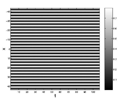
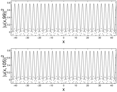
FIG. 1.: An example of evolution of the $A_{1}A_{2}$ double mode with equal amplitudes $\left|A_{1}\right|$ and $\left|A_{2}\right|$ in the case of the $2\!:\!1\!:\!1$ subharmonic resonance, constructed as per Eq. (50) for $\kappa=\mu=1$, $V_{0}=0.1$, $g=h=0.025$, and $\alpha=0.02$. The left subplot shows the spatio-temporal evolution of $\left|\psi_{1}\right|^{2}$ by means of grayscale contour plots ($\left|\psi_{2}\right|^{2}$ behaves similarly). The right subplot displays snapshots of the field $\left|\psi_{1}\right|^{2}$ for $t=99$ (upper panel) and $t=105$ (lower panel). In these panels, the optical-lattice potential is also shown by a dashed line. The results have been obtained through numerical integration of Eqs. (5) in time.

The other $A_{1}A_{2}$ double-mode equilibrium has unequal components $A_{1}$ and $A_{2}$ [note that in the non-resonant case considered above, the double-mode equilibria, which are given by Eqs. (39) and by a $\pi/2$ phase shift thereof, always have equal nonzero components]:

$\displaystyle A_{1}^{2}+A_{2}^{2}=\frac{2(2\mu_{1}+V_{0})}{3g}>0\,,$

$$(A_{1},A_{2},B_{1},B_{2}) =\pm\left(\sqrt{\frac{2\mu_{1}+V_{0}}{3g}\pm\frac{1}{3}\sqrt{\frac{(2\mu_{1}+V_{0})^{2}}{g^{2}}-\frac{16\alpha^{2}}{(g-h)^{2}}}}\,,\right.$$ (51)

$$\qquad\left.\sqrt{\frac{2\mu_{1}+V_{0}}{3g}\mp\frac{1}{3}\sqrt{\frac{(2\mu_{1}+V_{0})^{2}}{g^{2}}-\frac{16\alpha^{2}}{(g-h)^{2}}}},0,0\right)\,,$$ (52)

where the interior $+$ sign in the first component corresponds to the $-$ sign in the second, and vice versa. The exterior sign $\pm$ is independent of the interior one. A necessary condition for the existence of this solution is

$\displaystyle\left|\frac{2\mu_{1}+V_{0}}{g}\right|\geq\frac{4\alpha}{|g-h|}\,.$

In particular, when $h=2g$, which is a case of special physical relevance (as explained above), the solution becomes

$$(A_{1},A_{2},B_{1},B_{2}) =\pm\left(\sqrt{\frac{1}{3g}\left[2\mu_{1}+V_{0}\pm\sqrt{(2\mu_{1}+V_{0})^{2}-16\alpha^{2}}\right]}\,,\right.$$ (53)

$$\qquad\left.\sqrt{\frac{1}{3g}\left[2\mu_{1}+V_{0}\mp\sqrt{(2\mu_{1}+V_{0})^{2}-16\alpha^{2}}\right]},0,0\right)\,,$$ (54)

provided $|2\mu_{1}+V_{0}|\geq 4\alpha$.

In fact, the existence of pairs of equilibria in which the two components have unequal amplitudes that are mirror images of each other is a manifestation of spontaneous symmetry breaking in the present model, which is described by the symmetric system of coupled equations (5). A similar phenomenon was studied in detail (in terms of soliton solutions) in the aforementioned model of dual-core nonlinear optical fibers, which includes only linear coupling between two equations [33].

The stability of the asymmetric stationary solutions, which correspond to equilibria with unequal components, was also simulated in the framework of Eqs. (5). We show the results of a typical simulation in Fig. 2. As seen in the figure, these states are subject to periodic oscillations between the two components (which is possible only in the presence of the linear coupling between them).

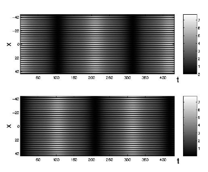
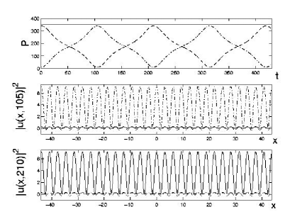
FIG. 2.: The same as in Fig. 1, but for the $A_{1}A_{2}$ double mode with unequal amplitudes $\left|A_{1}\right|$ and $\left|A_{2}\right|$, given by Eq. (52). The top panel in the right subplot shows the time evolution of the numbers of atoms in the two components, $N_{1,2}=\int|\psi_{1,2}|^{2}dx$, by dashed and dash-dotted lines (the sum of the two, $N=N_{1}+N_{2}$, is shown by the solid line). The right panel also shows the fields $\left|\psi_{1}\right|^{2}$ and $\left|\psi_{2}\right|^{2}$ (by solid and dash-dotted lines, respectively) at $t=105$ and $t=210$. The OL potential is shown by the dashed line. Oscillations of matter between the two components are clearly discernible. The parameters are $g=0.025$, $h=0.005$, $\alpha=-0.02$, $V_{0}=0.3$, and $\kappa=\mu=1$. (Recall that the sign of $\alpha$ can be chosen arbitrarily.)

The resonant equations (48) give rise to two types of $B_{1}B_{2}$ dual-mode equilibria. The first satisfies $B_{1}^{2}=B_{2}^{2}$ and

$$(A_{1},A_{2},B_{1},B_{2}) =\pm\left(0,0,\sqrt{\frac{-4\alpha+2(2\mu_{1}-V_{0})}{3(g+h)}},\sqrt{\frac{-4\alpha+2(2\mu_{1}-V_{0})}{3(g+h)}}\right)\,,$$ (55)

$$(A_{1},A_{2},B_{1},B_{2}) =\pm\left(0,0,\sqrt{\frac{4\alpha+2(2\mu_{1}-V_{0})}{3(g+h)}},-\sqrt{\frac{4\alpha+2(2\mu_{1}-V_{0})}{3(g+h)}}\right)\,.$$ (56)

The second type satisfies

$\displaystyle B_{1}^{2}+B_{2}^{2}=\frac{2(2\mu_{1}-V_{0})}{3g}>0\,,$

$$(A_{1},A_{2},B_{1},B_{2}) =\pm\left(0,0,\sqrt{\frac{2\mu_{1}-V_{0}}{3g}\pm\frac{1}{3}\sqrt{\frac{(2\mu_{1}-V_{0})^{2}}{g^{2}}-\frac{16\alpha^{2}}{(g-h)^{2}}}},\right.$$ (57)

$$\qquad\left.\sqrt{\frac{2\mu_{1}-V_{0}}{3g}\mp\frac{1}{3}\sqrt{\frac{(2\mu_{1}-V_{0})^{2}}{g^{2}}-\frac{16\alpha^{2}}{(g-h)^{2}}}}\right)\,.$$ (58)

As above, the interior $+$ sign in the first component is paired to the $-$ sign in the second, and vice versa, whereas the exterior $\pm$ is independent. A necessary condition for the existence of this solution is

$$\left|\frac{2\mu_{1}-V_{0}}{g}\right|\geq\frac{4\alpha}{|g-h|}\,.$$ (59)

When $h=2g$, the present solution becomes

$$(A_{1},A_{2},B_{1},B_{2}) =\pm\left(0,0,\sqrt{\frac{1}{3g}\left[2\mu_{1}-V_{0}\pm\sqrt{(2\mu_{1}-V_{0})^{2}-16\alpha^{2}}\right]},\right.$$ (60)

$$\qquad\left.\sqrt{\frac{1}{3g}\left[2\mu_{1}-V_{0}\mp\sqrt{(2\mu_{1}-V_{0})^{2}-16\alpha^{2}}\right]}\right)\,,$$ (61)

provided $|2\mu_{1}-V_{0}|\geq 4\alpha$.

Unlike the non-resonant case, the resonant $B_{1}B_{2}$ modes are not precise phase shifts of the $A_{1}A_{2}$ modes, as the spatial parametric excitation resulting from the OL has only the cosine harmonic. Nevertheless, the equations describing these two classes of modes are similar, differing only in the sign of $V_{0}$. Direct simulations demonstrate that the stability of stationary solutions corresponding to the $B_{1}B_{2}$ equilibria is the same as in the case of the $A_{1}A_{2}$ double-mode equilibria considered above: the symmetric ones with $\left|B_{1}\right|=\left|B_{2}\right|$ are stable, and the asymmetric solutions with $\left|B_{1}\right|\neq\left|B_{2}\right|$ are unstable.

We have also found two sets of quadruple modes in the resonant case. The first set satisfies $B_{1}=B_{2}$, $A_{1}=-A_{2}$, and

$$A_{1}^{2} =\frac{V_{0}}{2h}+\frac{\alpha}{h}+\frac{2\mu_{1}}{3g+h},$$ (62)

$$B_{1}^{2} =-\frac{V_{0}}{2h}-\frac{\alpha}{h}+\frac{2\mu_{1}}{3g+h}\,.$$ (63)

A necessary condition for its existence is

$\displaystyle\frac{2\mu_{1}}{3g+h}>\left|\frac{V_{0}}{2h}+\frac{\alpha}{h}\right|\,,$

and hence it is necessary that $\mu_{1}/(3g+h)>0$. The second set of quadruple modes satisfies $B_{1}=-B_{2}$, $A_{1}=A_{2}$, and

$$A_{1}^{2} =\frac{V_{0}}{2h}-\frac{\alpha}{h}+\frac{2\mu_{1}}{3g+h}\,,$$ (64)

$$B_{1}^{2} =-\frac{V_{0}}{2h}+\frac{\alpha}{h}+\frac{2\mu_{1}}{3g+h}\,.$$ (65)

A necessary existence condition for this mode to exist is

$\displaystyle\frac{2\mu_{1}}{3g+h}>\left|\frac{V_{0}}{2h}-\frac{\alpha}{h}\right|\,,$

which also implies that $\mu_{1}/(3g+h)>0$.

We considered quadruple modes in the presence of detuning, so $\mu_{1}\neq 0$. This is rather difficult to implement numerically, as—in view of the periodic boundary conditions in $x$ employed in the numerical integration scheme—it is necessary to match both the potential and initial condition to the size of the integration domain. Nevertheless, we were able to perform stability simulations in this case too. We show an example of these simulations in Fig. 3. We observe that the quadruple mode is unstable against long-wave perturbations, even if the simulations are run with $\alpha=0$ (no linear coupling). We have not observed stable quadruple states.

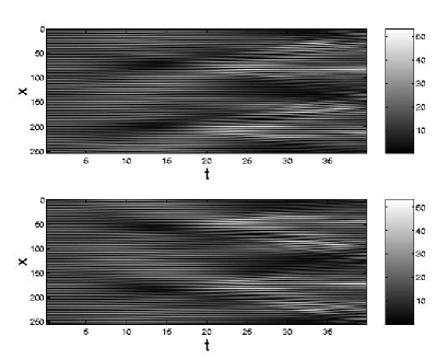
FIG. 3.: A typical example of the long-wave instability of a quadruple (four-amplitude) stationary state in the resonant case. The parameters are $\mu=1.5791$, $\kappa=1.2320$, $V_{0}=0.1$, $g=0.025$, $h=0.05$ and $\alpha=0$, and the size of the integration box is $L=255$.

When $\alpha=0$ (no linear coupling between BEC components), one can find additional double-mode equilibria and four single-mode ones, the latter of which take the form $(A_{1},0,0,0)$, $(0,A_{2},0,0)$, $(0,0,B_{1},0)$, $(0,0,0,B_{2})$, with

$$A_{1}^{2} =A_{2}^{2}=\frac{2(2\mu_{1}+V_{0})}{3g}>0\,,$$ (66)

$$B_{1}^{2} =B_{2}^{2}=-\frac{2(2\mu_{1}-V_{0})}{3g}>0\,.$$ (67)

The $A_{j}$- and $B_{j}$-modes both exist when $V_{0}/g>0$. In this case ($\alpha=0$), matter cannot be exchanged between the components. In this same situation, there is also an $A_{1}B_{2}$ double-mode equilibrium [of the form $(A_{1},0,0,B_{2})$], which satisfies

$$A_{1}^{2} =\frac{4\mu_{1}}{3g+h}+\frac{2V_{0}}{3g-h}>0\,,$$ (68)

$$B_{2}^{2} =\frac{4\mu_{1}}{3g+h}-\frac{2V_{0}}{3g-h}>0\,.$$ (69)

From Eq. (69), it follows that a necessary condition for this mode to exist is $8\mu_{1}/(3g+h)>0$. Its counterpart is an $A_{2}B_{1}$ equilibrium, in which the subscripts $1$ and $2$ are swapped in Eq. (69).

One can extend the analysis to higher-order spatial resonances in BECs (from the lowest subharmonic resonance considered here) either by considering higher-order corrections to the averaged equations, or by employing a perturbative scheme based on elliptic functions, as has been done for single-component BECs in OLs[39, 38]. Toward this aim, it may be fruitful to utilize an action-angle formulation and the elliptic-function structure of solutions to Eqs. (23) when $V_{0}=0$. However, detailed consideration of higher-order resonances is beyond the scope of this work.

V Ternary BECs in Optical Lattices

To evince the generality of the above analysis, we briefly consider its extension to a BEC model of three hyperfine states coupled by two different microwave fields, which is also a physically relevant situation [19]. The corresponding coupled GP equations (with $\hbar=1$ and $m=1/2$) are

$$i\frac{\partial\psi_{1}}{\partial t} =-\nabla^{2}\psi_{1}+g|\psi_{1}|^{2}\psi_{1}+V(x)\psi_{1}+h_{12}|\psi_{2}|^{2}\psi_{1}+h_{13}|\psi_{3}|^{2}\psi_{1}+\alpha_{12}\psi_{2}+\alpha_{13}\psi_{3}\,,$$ (70)

$$i\frac{\partial\psi_{2}}{\partial t} =-\nabla^{2}\psi_{2}+g|\psi_{2}|^{2}\psi_{2}+V(x)\psi_{2}+h_{12}|\psi_{1}|^{2}\psi_{2}+h_{23}|\psi_{3}|^{2}\psi_{2}+\alpha_{12}\psi_{1}+\alpha_{23}\psi_{3}\,,$$ (71)

$$i\frac{\partial\psi_{3}}{\partial t} =-\nabla^{2}\psi_{3}+g|\psi_{3}|^{3}\psi_{3}+V(x)\psi_{3}+h_{13}|\psi_{1}|^{2}\psi_{3}+h_{23}|\psi_{2}|^{2}\psi_{3}+\alpha_{13}\psi_{1}+\alpha_{23}\psi_{2}\,,$$ (72)

where the self- and cross-scattering coefficients are $g:=g_{1}=g_{2}=g_{3}$ and $h_{jk}$, and the linear coupling constants are $\alpha_{jk}$.

As in the binary case, we start with the general form (14) for stationary solutions, with $\theta_{1}(x)=\theta_{2}(x)=\theta_{3}(x)\equiv\theta(x)$ and $\mu_{1}=\mu_{2}=\mu_{3}\equiv\mu$. Then, as done above, we set $c_{j}=0$ (i.e., $\theta=0$) in Eqs. (19) to consider standing wave solutions and arrive at the following equations:

$$R_{1}^{\prime} =S_{1}\,,$$ (73)

$$S_{1}^{\prime} =-\mu R_{1}+gR_{1}^{3}+h_{12}R_{1}R_{2}^{2}+h_{13}R_{1}R_{3}^{2}+\alpha_{12}R_{2}+\alpha_{13}R_{3}+V(x)R_{1}\,,$$ (74)

$$R_{2}^{\prime} =S_{2}\,,$$ (75)

$$S_{2}^{\prime} =-\mu R_{2}+gR_{2}^{3}+h_{12}R_{1}^{2}R_{2}+h_{23}R_{2}R_{3}^{2}+\alpha_{12}R_{1}+\alpha_{23}R_{3}+V(x)R_{2}\,,$$ (76)

$$R_{3}^{\prime} =S_{3}\,,$$ (77)

$$S_{3}^{\prime} =-\mu R_{3}+gR_{3}^{3}+h_{13}R_{1}^{2}R_{3}+h_{23}R_{2}^{2}R_{3}+\alpha_{13}R_{1}+\alpha_{23}R_{2}+V(x)R_{3}\,,$$ (78)

where $V(x)$ is the sinusoidal OL potential, as before.

One can average Eqs. (78) with the same procedure that we applied to Eqs. (23) and thereby derive both resonant and non-resonant equations describing the system’s slow dynamics. In particular, for the most fundamental resonant case (the lowest-order, $2\!:\!1\!:\!1\!:\!1$, resonance), the averaged equations are

$$A_{1}^{\prime} =\frac{\epsilon}{\kappa}\left[\left(\frac{\tilde{\mu}_{1}}{2}-\frac{\tilde{V}_{0}}{4}\right)B_{1}-\frac{3\tilde{g}}{8}B_{1}(A_{1}^{2}+B_{1}^{2})-\frac{\tilde{\alpha}_{12}}{2}B_{2}-\frac{\tilde{\alpha}_{13}}{2}B_{3}-\frac{\tilde{h}_{12}}{4}A_{1}A_{2}B_{2}-\frac{\tilde{h}_{13}}{4}A_{1}A_{3}B_{3}\right.$$ (79)

$$\qquad\left.-\frac{\tilde{h}_{12}}{8}B_{1}(A_{2}^{2}+3B_{2}^{2})-\frac{\tilde{h}_{13}}{8}B_{1}(A_{3}^{2}+3B_{3}^{2})\right]+O(\epsilon^{2})\,,$$ (80)

$$A_{2}^{\prime} =\frac{\epsilon}{\kappa}\left[\left(\frac{\tilde{\mu}_{1}}{2}-\frac{\tilde{V}_{0}}{4}\right)B_{2}-\frac{3\tilde{g}}{8}B_{2}(A_{2}^{2}+B_{2}^{2})-\frac{\tilde{\alpha}_{12}}{2}B_{1}-\frac{\tilde{\alpha}_{23}}{2}B_{3}-\frac{\tilde{h}_{12}}{4}A_{1}A_{2}B_{1}-\frac{\tilde{h}_{23}}{4}A_{2}A_{3}B_{3}\right.$$ (81)

$$\qquad\left.-\frac{\tilde{h}_{12}}{8}B_{2}(A_{1}^{2}+3B_{1}^{2})-\frac{\tilde{h}_{23}}{8}B_{2}(A_{3}^{2}+3B_{3}^{2})\right]+O(\epsilon^{2})\,,$$ (82)

$$A_{3}^{\prime} =\frac{\epsilon}{\kappa}\left[\left(\frac{\tilde{\mu}_{1}}{2}-\frac{\tilde{V}_{0}}{4}\right)B_{3}-\frac{3\tilde{g}}{8}B_{3}(A_{3}^{2}+B_{3}^{2})-\frac{\tilde{\alpha}_{13}}{2}B_{1}-\frac{\tilde{\alpha}_{23}}{2}B_{2}-\frac{\tilde{h}_{13}}{4}A_{1}A_{3}B_{1}-\frac{\tilde{h}_{23}}{4}A_{2}A_{3}B_{2}\right.$$ (83)

$$\qquad\left.-\frac{\tilde{h}_{13}}{8}B_{3}(A_{1}^{2}+3B_{1}^{2})-\frac{\tilde{h}_{23}}{8}B_{3}(A_{2}^{2}+3B_{2}^{2})\right]+O(\epsilon^{2})\,,$$ (84)

$$B_{1}^{\prime} =\frac{\epsilon}{\kappa}\left[-\left(\frac{\tilde{\mu}_{1}}{2}+\frac{\tilde{V}_{0}}{4}\right)A_{1}+\frac{3\tilde{g}}{8}A_{1}(A_{1}^{2}+B_{1}^{2})+\frac{\tilde{\alpha}_{12}}{2}A_{2}+\frac{\tilde{\alpha}_{13}}{2}A_{3}+\frac{\tilde{h}_{12}}{4}A_{2}B_{1}B_{2}+\frac{\tilde{h}_{13}}{4}A_{3}B_{1}B_{3}\right.$$ (85)

$$\qquad\left.+\frac{\tilde{h}_{12}}{8}A_{1}(3A_{2}^{2}+B_{2}^{2})+\frac{\tilde{h}_{13}}{8}A_{1}(3A_{3}^{2}+B_{3}^{2})\right]+O(\epsilon^{2})\,,$$ (86)

$$B_{2}^{\prime} =\frac{\epsilon}{\kappa}\left[-\left(\frac{\tilde{\mu}_{1}}{2}+\frac{\tilde{V}_{0}}{4}\right)A_{2}+\frac{3\tilde{g}}{8}A_{2}(A_{2}^{2}+B_{2}^{2})+\frac{\tilde{\alpha}_{12}}{2}A_{1}+\frac{\tilde{\alpha}_{23}}{2}A_{3}+\frac{\tilde{h}_{12}}{4}A_{1}B_{1}B_{2}+\frac{\tilde{h}_{23}}{4}A_{3}B_{2}B_{3}\right.$$ (87)

$$\qquad\left.+\frac{\tilde{h}_{12}}{8}A_{2}(3A_{1}^{2}+B_{1}^{2})+\frac{\tilde{h}_{23}}{8}A_{2}(3A_{3}^{2}+B_{3}^{2})\right]+O(\epsilon^{2})\,,$$ (88)

$$B_{3}^{\prime} =\frac{\epsilon}{\kappa}\left[-\left(\frac{\tilde{\mu}_{1}}{2}+\frac{\tilde{V}_{0}}{4}\right)A_{3}+\frac{3\tilde{g}}{8}A_{3}(A_{3}^{2}+B_{3}^{2})+\frac{\tilde{\alpha}_{13}}{2}A_{1}+\frac{\tilde{\alpha}_{23}}{2}A_{2}+\frac{\tilde{h}_{13}}{4}A_{1}B_{1}B_{3}+\frac{\tilde{h}_{23}}{4}A_{2}B_{2}B_{3}\right.$$ (89)

$$\qquad\left.+\frac{\tilde{h}_{13}}{8}A_{3}(3A_{1}^{2}+B_{1}^{2})+\frac{\tilde{h}_{23}}{8}A_{3}(3A_{2}^{2}+B_{2}^{2})\right]+O(\epsilon^{2})\,.$$ (90)

One can find double-mode solutions to (90) that are analogous to those of Eq. (48). For example, if $|\alpha_{13}|=|\alpha_{23}|$, so that the first and second components in the ternary condensate have the same strength in their linear coupling to the third component, there exists a double-mode equilibrium with $A_{1}^{2}=A_{2}^{2}$ and $A_{3}=B_{1}=B_{2}=B_{3}=0$. The values of $A_{1}$ and $A_{2}$ are exactly as for binary BECs [see Eq. (50)], except that $\alpha$ and $h$ in the solution are replaced by $\alpha_{12}$ and $h_{12}$. Further, in this case, one finds $A_{1}=-A_{2}$ for $\alpha_{13}=\alpha_{23}$ and $A_{1}=A_{2}$ for $\alpha_{13}=-\alpha_{23}$. In fact, these modes are a straightforward extension of their two-component counterparts, as the third component is absent in the stationary solution. Furthermore, the stability of the symmetric double-mode equilibria, reported above, ensures the stability of these solutions in the ternary model.

The situation is more interesting for asymmetric two-mode solutions, such as the ones corresponding to Eq. (52), which are, simultaneously, solutions to Eqs. (72) with $A_{3}=B_{3}=0$, provided $A_{1}=-(\alpha_{23}/\alpha_{13})A_{2}$. [Note that this relation is used to determine $\alpha_{23}/\alpha_{13}$, as $A_{1}$ and $A_{2}$ are determined from Eq. (52).] Direct simulations of the three-component GP equations (72) with $h:=h_{12}=h_{13}=h_{23}$ show that these asymmetric solutions are unstable, just as in the two-component model. The instability development, illustrated by Fig. 4, leads to an interesting dynamical interplay between the components. In particular, as a result of the instability, the third component is eventually excited, which leads to periodic oscillation of matter between all three components; i.e., in this case, we observe a true example of three-component dynamics.

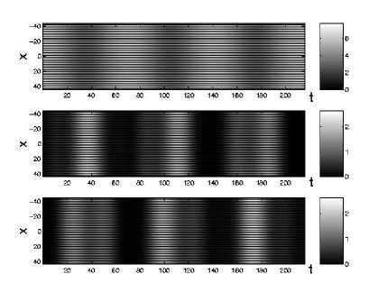
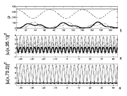
FIG. 4.: The same as in Fig. 2, but for the three-component (ternary) model. The bottom panel of the left plot shows the spatio-temporal evolution of the third component (which is absent in the unperturbed, unstable two-mode solution), and the thick solid line on the right shows the evolution of the number of atoms in this component (top subplot). Its spatial profile is shown as well (middle and bottom subplots, for $t=35.1$ and $t=70.2$, respectively). Periodic oscillations of matter between all three components are evident, cf. the oscillations in the two-compoment model, displayed in Fig. 2. The parameters are $g=0.025$, $h=0.005$, $\alpha_{12}=\alpha_{13}=-0.02$, $V_{0}=0.3$, and $\kappa=\mu=1$. The quantity $\alpha_{23}\approx 0.117$ is determined from the values of $\alpha_{12}=\alpha_{13}=-0.02$ (see text).

VI Conclusions

In this work, we analyzed spatial structures in coupled Gross-Pitaevskii (coupled GP) equations, which include both nonlinear and linear interactions, in an optical-lattice (OL) potential. The model describes a BEC consisting of a mixture of two different hyperfine states of one atomic species, which are linearly coupled by a resonant electromagnetic field. In the absence of the OL, we found plane-wave solutions and examined their stability. In the presence of the OL, we derived a system of averaged equations to describe a spatially modulated state which is coupled to the periodic potential through a subharmonic resonance. We found equilibria of the latter system and examined the stability of the corresponding spatially periodic solutions to the coupled GP equations using direct simulations. We demonstrated that symmetric dual-mode resonant states with two equal amplitudes are stable, whereas asymmetric ones (with unequal amplitudes) are unstable, generating solutions that oscillate periodically in time. The latter type of dynamical behavior is only possible in the presence of linear coupling between BEC components. We found four-mode stationary solutions as well, but they are always unstable. Finally, a three-component generalization of the model was introduced and briefly considered. In this case, we found that the unstable asymmetric two-mode solution, with one component originally empty, develops time-periodic oscillations in which the initially empty component becomes populated.

Appendix

The functions $F_{A_{j}}$ and $F_{B_{j}}$, which appear in Eqs. (30), can be written as a sum of harmonic contributions. To simplify the notation, we write $\tilde{g}$, $\tilde{h}$, $\tilde{\alpha}$, and $\tilde{V}_{0}$ simply as $g$, $h$, $\alpha$, and $V$.

In the non-resonant case, $F_{A_{1}}=G_{A_{1}}/\sqrt{\mu}$, where

$$G_{A_{1}}(A_{1},A_{2},A_{3},A_{4},x) =\left[-\frac{\alpha}{2}-\frac{3g}{8}B_{1}(A_{1}^{2}+B_{1}^{2})-\frac{h}{4}A_{1}A_{2}B_{2}-\frac{h}{8}B_{1}(A_{2}^{2}+3B_{2}^{2})\right]$$ (91)

$$\quad+\left[-\frac{\alpha}{2}-\frac{g}{4}A_{1}(A_{1}^{2}+3B_{1}^{2})-\frac{h}{2}A_{2}B_{1}B_{2}-\frac{h}{4}A_{1}(A_{2}^{2}+B_{2}^{2})\right]\sin(2\sqrt{\mu}x)$$ (92)

$$\quad+\left[\frac{g}{8}A_{1}(3B_{1}^{2}-A_{1}^{2})+\frac{h}{4}A_{1}B_{1}B_{2}+\frac{h}{8}A_{1}(B_{2}^{2}-A_{2}^{2})\right]\sin(4\sqrt{\mu}x)$$ (93)

$$\quad+\left[-\frac{V}{4}A_{1}\right]\sin(2[\kappa-\sqrt{\mu}]x)+\left[\frac{V}{4}\right]\sin(2[\kappa+\sqrt{\mu}]x)$$ (94)

$$\quad+\left[\frac{g}{2}B_{1}^{3}+\frac{\alpha}{2}B_{2}+\frac{h}{2}B_{1}B_{2}^{2}\right]\cos(2\sqrt{\mu}x)$$ (95)

$$\quad+\left[\frac{g}{8}B_{1}(3A_{1}^{2}-B_{1}^{2})+\frac{h}{4}A_{1}A_{2}B_{2}+\frac{h}{8}B_{1}(A_{2}^{2}-B_{2}^{2})\right]\cos(4\sqrt{\mu}x)$$ (96)

$$\quad+\left[\frac{V}{2}B_{1}\right]\cos(2\kappa x)+\left[-\frac{V}{4}\right]\cos(2[\kappa-\sqrt{\mu}]x)+\left[-\frac{V}{4}\right]\cos(2[\kappa+\sqrt{\mu}]x)\,,$$ (97)

and $F_{B_{1}}=G_{B_{1}}/\sqrt{\mu}$, where

$$G_{B_{1}}(A_{1},A_{2},A_{3},A_{4},x) =\left[\frac{\alpha}{2}A_{2}+\frac{3g}{8}A_{1}(A_{1}^{2}+B_{1}^{2})+\frac{h}{4}A_{2}B_{1}B_{2}+\frac{h}{8}A_{1}(A_{2}^{2}+B_{2}^{2})\right]$$ (98)

$$\quad+\left[\frac{\alpha}{2}B_{2}+\frac{g}{4}B_{1}(3A_{1}^{2}+B_{1}^{2})+\frac{h}{2}A_{1}A_{2}B_{2}+\frac{h}{4}B_{1}(A_{2}^{2}+B_{2}^{2})\right]\sin(2\sqrt{\mu}x)$$ (99)

$$\quad+\left[\frac{g}{8}B_{1}(3A_{1}^{2}-B_{1}^{2})+\frac{h}{4}A_{1}A_{2}B_{2}+\frac{h}{8}B_{1}(A_{2}^{2}-B_{2}^{2})\right]\sin(4\sqrt{\mu}x)$$ (100)

$$\quad+\left[\frac{V}{4}B_{1}\right]\sin(2[\kappa-\sqrt{\mu}]x)+\left[-\frac{V}{4}\right]\sin(2[\kappa+\sqrt{\mu}]x)$$ (101)

$$\quad+\left[\frac{\alpha}{2}A_{2}+\frac{g}{2}A_{1}^{3}+\frac{h}{2}A_{1}A_{2}^{2}\right]\cos(2\sqrt{\mu}x)$$ (102)

$$\quad+\left[\frac{g}{8}A_{1}(A_{1}^{2}-3B_{1}^{2})-\frac{h}{4}A_{2}B_{1}B_{2}+\frac{h}{8}A_{1}(A_{2}^{2}-B_{2}^{2})\right]\cos(4\sqrt{\mu}x)$$ (103)

$$\quad+\left[-\frac{V}{2}A_{1}\right]\cos(2\kappa x)+\left[-\frac{V}{4}A_{1}\right]\cos(2[\kappa-\sqrt{\mu}]x)+\left[-\frac{V}{4}A_{1}\right]\cos(2[\kappa+\sqrt{\mu}]x)\,.$$ (104)

Only $O(1)$ [i.e., constant harmonic] terms remain after averaging.

In the resonant case, one obtains, after averaging, an extra term depending on the periodic potential $V$, because a term that was a prefactor of a non-constant harmonic in (97) and (104) has become a coefficient in front of the $O(1)$ term. Other harmonic terms are also simplified due to the resonance, but they nevertheless do not contribute to the averaged equations because they are still prefactors of non-constant harmonics. The extra terms with $\mu_{1}$ arise from Taylor expanding in powers of $\epsilon$ and keeping the leading-order terms. In the resonant case, $F_{A_{1}}=G_{A_{1}}/\kappa$ and $F_{B_{1}}=G_{B_{1}}/\kappa$.

In both the resonant and non-resonant cases, the expressions for $F_{A_{2}}$ and $F_{B_{2}}$ are obtained by switching the subscripts $1\longleftrightarrow 2$ in the equations above.

REFERENCES

- [1] G. P. Agrawal. Nonlinear Fiber Optics. Academic Press, San Diego, CA, 1995.
- [2] G. L. Alfimov, P. G. Kevrekidis, V. V. Konotop, and M. Salerno. Wannier functions analysis of the nonlinear Schrodinger equation with a periodic potential. Physical Review E, 66(046608), October 2002.
- [3] B. P. Anderson and M. A. Kasevich. Macroscopic quantum interference from atomic tunnel arrays. Science, 282(5394):1686–1689, November 1998.
- [4] B. B. Baizakov, V. V. Konotop, and M. Salerno. Regular spatial structures in arrays of Bose-Einstein condensates induced by modulational instability. Journal of Physics B: Atomic Molecular and Optical Physics, 35:5105–5119, 2002.
- [5] R. J. Ballagh, K. Burnett, and Scott T. F. Theory of an output coupler for Bose-Einstein condensed atoms. Physical Review Letters, 78:1607–1611, March 1997.
- [6] Y. B. Band, I. Towers, and Boris A. Malomed. Unified semiclassical approximation for Bose-Einstein condensates: Application to a BEC in an optical potential. Physical Review A, 67(023602), February 2003.
- [7] Kirstine Berg-Sørensen and Klaus Mølmer. Bose-Einstein condensates in spatially periodic potentials. Physical Review A, 58(2):1480–1484, August 1998.
- [8] Jared C. Bronski, Lincoln D. Carr, Ricardo Carretero-González, Bernard Deconinck, J. Nathan Kutz, and Keith Promislow. Stability of attractive Bose-Einstein condensates in a periodic potential. Physical Review E, 64(056615), 2001.
- [9] Jared C. Bronski, Lincoln D. Carr, Bernard Deconinck, and J. Nathan Kutz. Bose-Einstein condensates in standing waves: The cubic nonlinear Schrödinger equation with a periodic potential. Physical Review Letters, 86(8):1402–1405, February 2001.
- [10] Jared C. Bronski, Lincoln D. Carr, Bernard Deconinck, J. Nathan Kutz, and Keith Promislow. Stability of repulsive Bose-Einstein condensates in a periodic potential. Physical Review E, 63(036612), 2001.
- [11] S. Burger, F. S. Cataliotti, C. Fort, F. Minardi, and M. Inguscio. Superfluid and dissipative dynamics of a Bose-Einstein condensate in a periodic optical potential. Physical Review Letters, 86(20):4447–4450, May 2001.
- [12] Keith Burnett, Mark Edwards, and Charles W. Clark. The theory of Bose-Einstein condensation of dilute gases. Physics Today, 52(12):37–42, December 1999.
- [13] Th. Busch, J. I. Cirac, V. M. Pérez-García, and P. Zoller. Stability and collective excitations of a two-component Bose-Einstein condensed gas: A moment approach. Physical Review A, 56(4):2978–2983, October 1997.
- [14] Ricardo Carretero-González and Keith Promislow. Localized breathing oscillations of Bose-Einstein condensates in periodic traps. Physical Review A, 66(033610), September 2002.
- [15] Dae-Il Choi and Qian Niu. Bose-Einstein condensates in an optical lattice. Physical Review Letters, 82(10):2022–2025, March 1999.
- [16] Franco Dalfovo, Stefano Giorgini, Lev P. Pitaevskii, and Sandro Stringari. Theory of Bose-Einstein condensation on trapped gases. Reviews of Modern Physics, 71(3):463–512, April 1999.
- [17] Bernard Deconinck, B. A. Frigyik, and J. Nathan Kutz. Dynamics and stability of Bose-Einstein condensates: The nonlinear Schrödinger equation with periodic potential. Journal of Nonlinear Science, 12(3):169–205, 2002.
- [18] Bernard Deconinck, J. Nathan Kutz, Matthew S. Patterson, and Brandon W. Warner. Dynamics of periodic multi-component Bose-Einstein condenates. Journal of Physics A–Mathematics and General, 36(20):5431–5447, May 2003.
- [19] P. Engels. Personal communication.
- [20] B. D. Esry, Chris H. Greene, James P. Burke Jr., and John L. Bohn. Hartree-Fock theory for double condensates. Physical Review Letters, 78(19):3594–3597, May 1997.
- [21] John Guckenheimer and Philip Holmes. Nonlinear Oscillations, Dynamical Systems, and Bifurcations of Vector Fields. Number 42 in Applied Mathematical Sciences. Springer-Verlag, New York, NY, 1983.
- [22] E. W. Hagley, L. Deng, M. Kozuma, J. Wen, K. Helmerson, S. L. Rolston, and W. D. Phillips. A well-collimated quasi-continuous atom laser. Science, 283(5408):1706–1709, March 1999.
- [23] D. S. Hall. Personal communication.
- [24] Tin-Lun Ho and V. B. Shenoy. Binary mixtures of Bose condensates of alkali atoms. Physical Review Letters, 77(16):3276–3279, October 1996.
- [25] S. Inouye, M. R. Andrews, J. Stenger, H. J. Miesner, D. M. Stamper-Kurn, and W. Ketterle. Observation of Feshbach resonances in a Bose-Einstein condensate. Nature, 392(6672):151–154, March 1998.
- [26] Wolfgang Ketterle. Experimental studies of Bose-Einstein condensates. Physics Today, 52(12):30–35, December 1999.
- [27] Thorsten Köhler. Three-body problem in a dilute Bose-Einstein condensate. Physical Review Letters, 89(21):210404, 2002.
- [28] Anatoly Kuklov, Nikolay Prokof’ev, and Boris Svistunov. Detecting supercounterfluidity by Ramsey spectroscopy. Physical Review A, 69(025601), February 2004.
- [29] Pearl J. Y. Louis, Elena A. Ostrovskaya, Craig M. Savage, and Yuri S. Kivshar. Bose-einstein condensates in optical lattices: Band-gap structure and solitons. Physical Review A, 67(013602), 2003.
- [30] M. Machholm, A. Nicolin, C. J. Pethick, and H. Smith. Spatial period-doubling in Bose-Einstein condensates in an optical lattice. Physical Review A, 69(043604), 2004. ArXiv:cond-mat/0307183.
- [31] M. Machholm, C. J. Pethick, and H. Smith. Band structure, elementary excitations, and stability of a Bose-Einstein condensate in a periodic potential. Physical Review A, 67(053613), 2003.
- [32] Boris A. Malomed. Polarization dynamics and interactions of solitons in a birefringent optical fiber. Physical Review A, 43(1):410–423, January 1991.
- [33] Boris A. Malomed, I. M. Skinner, P. L. Chu, and G. D. Peng. Symmetric and asymmetric solitons in twin-core nonlinear optical fibers. Physical Review E, 53(4):4084–4091, April 1996.
- [34] Boris A. Malomed, Z. H. Wang, P. L. Chu, and G. D. Peng. Multichannel switchable system for spatial solitons. Journal of the Optical Society of America B, 16(8):1197–1203, August 1999.
- [35] Erich J. Mueller. Superfluidity and mean-field energy loops; hysteretic behavior in Bose-Einstein condensates. Physical Review A, 66(063603), 2002.
- [36] C. J. Myatt, E. A. Burt, R. W. Ghrist, E. A. Cornell, and C. E. Wieman. Production of two overlapping Bose-Einstein condensates by sympathetic cooling. Physical Review Letters, 78:586–589, January 1997.
- [37] C. J. Pethick and H. Smith. Bose-Einstein Condensation in Dilute Gases. Cambridge University Press, Cambridge, United Kingdom, 2002.
- [38] Mason A. Porter and Predrag Cvitanović. Modulated amplitude waves in Bose-Einstein condensates. Physical Review E, 69(047201), 2004. ArXiv: nlin.CD/0307032.
- [39] Mason A. Porter and Predrag Cvitanović. A perturbative analysis of modulated amplitude waves in Bose-Einstein condensates. Chaos, To appear. ArXiv: nlin.CD/0308024.
- [40] H. Pu and N. P. Bigelow. Collective excitations, metastability, and nonlinear response of a trapped two-species Bose-Einstein condensate. Physical Review Letters, 80(6):1134–1137, February 1998.
- [41] H. Pu and N. P. Bigelow. Properties of two-species Bose condensates. Physical Review Letters, 80(6):1130–1133, February 1998.
- [42] Richard H. Rand. Topics in Nonlinear Dynamics with Computer Algebra, volume 1 of Computation in Education: Mathematics, Science and Engineering. Gordon and Breach Science Publishers, USA, 1994.
- [43] Richard H. Rand. Dynamics of a nonlinear parametrically-excited pde: 2-term truncation. Mechanics Research Communications, 23(3):283–289, 1996.
- [44] Richard H. Rand. Lecture notes on nonlinear vibrations. a free online book available at http://www.tam.cornell.edu/randdocs/nlvibe45.pdf, 2003.
- [45] L. Salasnich, A. Parola, and L. Reatto. Periodic quantum tunnelling and parametric resonance with cigar-shaped Bose-Einstein condensates. Journal of Physics B: Atomic Molecular and Optical Physics, 35(14):3205–3216, July 2002.
- [46] D. T. Son and M. A. Stephanov. Domain walls of relative phase in two-component Bose-Einstein condensates. Physical Review A, 65:063621, June 2002.
- [47] Marek Trippenbach, Krzysztof Góral, Kazimierz Rza̧żewski, Boris Malomed, and Y. B. Band. Structure of binary Bose-Einstein condensates. Journal of Physics B: Atomic, Molecular, and Optical Physics, 33:4017–4031, 2000.
- [48] A. Trombettoni and A. Smerzi. Discrete solitons and breathers with dilute Bose-Einstein condensates. Physical Review Letters, 86(11):2353–2356, March 2001.
- [49] J. A. C. Weideman and B. M. Herbst. Split-step methods for the solution of the nonlinear Schrödinger equation. SIAM Journal on Numerical Analysis, 23(3):485–507, June 1986.
- [50] Biao Wu, Roberto B. Diener, and Qian Niu. Bloch waves and Bloch Bands of Bose-Einstein condensates in optical lattices. Physical Review A, 65(025601), 2002.