Consistent nonlinear dynamics: identifying model inadequacy

Abstract

Empirical modelling often aims for the simplest model consistent with the data. A new technique is presented which quantifies the consistency of the model dynamics as a function of location in state space. As is well-known, traditional statistics of nonlinear models like root-mean-square (RMS) forecast error can prove misleading. Testing consistency is shown to overcome some of the deficiencies of RMS error, both within the perfect model scenario and when applied to data from several physical systems using previously published models. In particular, testing for consistent nonlinear dynamics provides insight towards (i) identifying when a delay reconstruction fails to be an embedding, (ii) allowing state dependent model selection and (iii) optimising local neighbourhood size. It also provides a more relevant (state dependent) threshold for identifying false nearest neighbours.

url]http://www.cats.lse.ac.uk

1 Introduction

The construction of mathematical models whose dynamics reflect the observations of physical systems is arguably the fundamental task of physics [1]. A model’s ability to reproduce the observed dynamics is often quantified through the distribution of forecast errors. Indeed in traditional time series analysis the “optimal model” is defined as that which minimises the root-mean-square (RMS) error [2]. For a nonlinear system, this approach has the undesirable property that it may reject the model which generated the data. In this paper, a new test is introduced which quantifies the level of consistency between each iteration of the model and the observations; this test is of particular value for nonlinear models where uncertainty in the data due to observational noise limits the utility of statistics like RMS error [2, 3, 4]. Ideally, a model will admit trajectories which shadow the entire dataset to within the limits set by observational noise [4, 5, 6]; testing for consistent nonlinear dynamics (CND) provides a simple, computationally tractable, necessary condition for shadowing. The CND approach is applicable to models based on first principles [7, 8] and data-based empirical models [9, 10, 11, 12, 13, 14]. The aim is to confirm the simplest model consistent with the data, but none simpler.

As a test of the dynamics, the CND approach quantifies consistency as a function of location in model-state space. It is novel in that it (i) identifies regions where the model is notably imperfect, (ii) can suggest regions where an embedding fails (that is, where no deterministic model is consistent), (iii) provides a rational for setting a (local) threshold for the method of false nearest neighbours [15], and (iv) provides a means of selecting and weighting models for multi-model ensemble prediction [4, 7]. Models may be either linear or nonlinear, and the results below are easily generalised to stochastic models [2, 16], although the discussion here is restricted to the case of deterministic models and additive observational noise. While most of the examples below evaluate data-based empirical models, the consistent nonlinear dynamics approach is applicable to any dynamical model: it evaluates the particular model along with background modelling assumptions such as stationarity and the assumed form of observational noise.

Basic goals and methodology are presented in Section 2. Section 3 provides a brief and selective review of data-based model building in delay space. Two mathematical systems are then used to illustrate the method in section 4 and applications to previously published models of three widely studied physical systems, each thought to be chaotic, is given in section 5. The implications of these results for nonlinear modelling are discussed and interpreted in section 6 and conclusions are given in section 7.

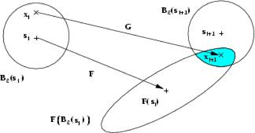
Figure 1: Consistent prediction: a trajectory of ${\bf G}$, with initial and final positions ${\bf x}$ ($\times$), corresponding observed positions ${\bf s}$ (+), their consistency balls, ${\cal B}_{\epsilon}({\bf s}_{i})$ and ${\cal B}_{\epsilon}({\bf s}_{i+1})$ (circles), and images of model-states which are consistent with ${\bf s}_{i}$, ${\bf F}\{{\cal B}_{\epsilon}({\bf s}_{i})\}$ (ellipse). The intersection of ${\bf F}\{{\cal B}_{\epsilon}({\bf s}_{i})\}$ with ${\cal B}_{\epsilon}({\bf s}_{i+1})$ signifies consistency.

2 Methodology

In this section, a constraint on state-dependent forecast error is derived; this forms the basic consistency test of CND. A number of simplifying assumptions are made to ease the derivation, often these can be relaxed and more general solutions deployed numerically (at the cost of simplicity and computational time).

The most common means for quantifying the quality of a model are based on the statistics of prediction errors [2] (for alternatives, see [3, 17, 18, 19]). Consider a model ${\bf F}$, with observations ${\bf s}_{i}\in{\rm I\kern-1.6pt{\rm R}}^{m_{s}}$ corresponding to system states ${\bf x}_{i}\in{\rm I\kern-1.6pt{\rm R}}^{m_{x}}$ of the ‘true’ deterministic system ${\bf G}$. Assume $m_{s}=m_{x}=m$ in the following. Also assume additive measurement errors $\mbox{\boldmath${\eta}$}_{i}$ (i.e. ${\bf s}_{i}={\bf x}_{i}+\mbox{\boldmath${\eta}$}_{i}$). In this case, the one-step prediction error may be decomposed as

$${\bf E}_{\rm pred} = {\bf s}_{i+1}-{\bf F}({\bf s}_{i})$$ (1)

$$= ({\bf x}_{i+1}+\mbox{\boldmath${\eta}$}_{i+1})-{\bf F}({\bf x}_{i}+\mbox{\boldmath${\eta}$}_{i})$$

$$= \left[{\bf G}({\bf x}_{i})-{\bf F}({\bf x}_{i})\right]+\left[\mbox{\boldmath${\eta}$}_{i+1}+{\bf F}({\bf x}_{i})-{\bf F}({\bf x}_{i}+\mbox{\boldmath${\eta}$}_{i})\right]$$

$$= {\bf E}_{\rm model}+{\bf E}_{\rm noise},$$

where ${\bf E}_{\rm model}$ represents model inadequacy and ${\bf E}_{\rm noise}$ represents error due to observational uncertainty. Viewing the prediction error ${\bf E}_{\rm pred}$ as a sum of these two distinct sources of error highlights three facts: (i) prediction errors may be due to noise alone, and need not arise from model error, (ii) model error is obscured by observational uncertainty, and can only be accurately assessed if this uncertainty is taken into account, and (iii) prediction errors may manifest extreme fluctuations throughout model-state space due to variations in model sensitivity. Note the similarity of this decomposition with that for “model drift” used in operational weather forecasting [8, 21].

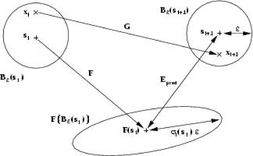
Figure 2: Inconsistent prediction: as Fig. 1. In this case no model trajectory exists which is consistent with the observational uncertainty since ${\bf F}\{{\cal B}_{\epsilon}({\bf s}_{i})\}$ does not intersect ${\cal B}_{\epsilon}({\bf s}_{i+1})$.

Prediction error due to additive noise in a perfect model may be expressed as a Taylor series:

$${\bf E}_{\rm noise}=\mbox{\boldmath${\eta}$}_{i+1}-{\bf J}({\bf x}_{i})\mbox{\boldmath${\eta}$}_{i}-\frac{1}{2}\mbox{\boldmath${\eta}$}^{T}_{i}{\bf H}({\bf x}_{i})\mbox{\boldmath${\eta}$}_{i}-\cdots$$ (2)

where ${\bf J}({\bf x})$ and ${\bf H}({\bf x})$ are the Jacobian and Hessian of ${\bf F}({\bf x})$. The distribution of ${\bf E}_{\rm noise}$ in (2) reflects how variations in the local derivatives of a particular model structure affects the local prediction error. When the distribution of $\mbox{\boldmath${\eta}$}_{i}$ is known, the distribution of ${\bf E}_{\rm noise}$ can be determined from (2) and, since ${\bf E}_{\rm pred}$ is known, regions of model-state space with large ${\bf E}_{\rm model}$ can be identified. Figures 1 and 2 illustrate this in model-state space where, for simplicity, the initial uncertainty is bounded (constrained to be within the circle) and the dynamics are locally linear (the circle evolves into an ellipse). The system state at initial time ${\bf x}_{i}$ and at final time ${\bf x}_{i+1}$ are marked by crosses. For model-state vectors ${\bf s}_{i}\in{\rm I\kern-1.6pt{\rm R}}^{m}$ and observational uncertainty uniformly distributed in a sphere of radius $\epsilon$, there exists an associated ball of consistent model-states ${\cal B}_{\epsilon}({\bf s}_{i})=\left\{\mbox{\boldmath${\xi}$}:\left|\left|\mbox{\boldmath${\xi}$}-{\bf s}_{i}\right|\right|\leq\epsilon\right\}$. In practice, only the observed positions ${\bf s}_{i}$ (pluses) and their associated consistency balls ${\cal B}_{\epsilon}({\bf s}_{i})$ (circles) are known. The consistency of a model’s forecast may be tested by evolving the ball ${\cal B}_{\epsilon}({\bf s}_{i})$ to the final time. This set of evolved states, ${\bf F}\{{\cal B}_{\epsilon}({\bf s}_{i})\}$, will resemble an ellipsoid if the evolution is locally linear (i.e. when $\epsilon$ is sufficiently small and ${\bf F}$ is sufficiently smooth). If ${\bf F}\{{\cal B}_{\epsilon}({\bf s}_{i})\}$ and ${\cal B}_{\epsilon}({\bf s}_{i+1})$ intersect, then the prediction is internally consistent (Fig. 1), otherwise it is deemed inconsistent (Fig. 2). The overlap of ${\bf F}\{{\cal B}_{\epsilon}({\bf s}_{i})\}$ and ${\cal B}_{\epsilon}({\bf s}_{i+1})$ implies the existence of a model trajectory which lies inside the ball ${\cal B}_{\epsilon}({\bf s}_{i})$ at the initial time and also inside the ball ${\cal B}_{\epsilon}({\bf s}_{i+1})$ at the final time; that trajectory is consistent with both the model dynamics and the observations.

The most pedestrian version of CND is simply to verify this necessary condition. The idea is simply to check whether the largest observational error in the worst direction is likely to account for the observations. In practice, obtaining ${\bf F}\{{\cal B}_{\epsilon}({\bf s}_{i})\}$ by propagating a ball of model-states in ${\rm I\kern-1.6pt{\rm R}}^{m}$ may prove to be computationally expensive. A first order approximation provides a linear consistency check which is easy to implement. The linear approximation of (2) is

$${\bf E}_{\rm noise}=\mbox{\boldmath${\eta}$}_{i+1}-{\bf J}({\bf x}_{i})\mbox{\boldmath${\eta}$}_{i}.$$ (3)

The first singular value, $\sigma_{1}({\bf s}_{i})$, of the Jacobian [4, 7] describes the largest possible (linear) magnification which corresponds to the major axis of ${\bf F}\{{\cal B}_{\epsilon}({\bf s}_{i})\}$. Note from Fig. 2 that there is no initial condition consistent under the model if the prediction error is greater than the magnitude of the major axis of ${\bf F}\{{\cal B}_{\epsilon}({\bf s}_{i})\}$ plus the radius of ${\cal B}_{\epsilon}({\bf s}_{i+1})$. If the noise level is large relative to the local curvature of the (model’s) solution manifold, then the linear approximation may be generalised for locally nonlinear models; for local linear models this result is exact.

The expected value of the observational noise divided by the (local) length scale at which quadratic terms become important provides a fundamental ratio for each local linear prediction; if this ratio is large one must consider local quadratic models. In regions where this ratio is small, and the length scale at which quadratic terms become important is also small relative to near neighbour distances, it is advantageous to take smaller neighbourhoods thereby improving the local linear model. CND can identify such regions.

Note that the details of the consistency test depends on the type of state space being employed. The state space may be constructed using either multivariate data or a delay reconstruction of univariate data. In the first case, each component of the model-state vector must be forecast and evaluated while in the case of the delay reconstruction only one component need be forecast, the others generated by a shift operator; this difference will have an impact on tests of CND. The type of uncertainty in the measurements may also be either bounded (e.g. truncation error) or unbounded (e.g. additive Gaussian noise). In the former, the initial observational uncertainty resulting from bounded measurement errors lies in a hyper-cube (that is, a box); given Gaussian noise, an isopleth of equal probability in the space will be a sphere (or an ellipse, depending on the metric adopted). The discussion below is framed in terms of quantization error, but this can easily be interpreted in terms of, say. the 99.9% isopleth of an unbounded noise distribution.

Many of the applications presented below assume a delay reconstructed state space with truncation errors in the observations, implying that ${\eta}$ is uniformly distributed inside a hyper-cube. The diagonal of any $m$-dimensional hyper-cube of side $\epsilon$ may be stretched to at most $\sigma_{1}({\bf s}_{i})\sqrt{m}\epsilon$ and uncertainty in the (scalar) verification implies an additional factor of $\epsilon$, so that the consistency measure is

$${\cal C}({\bf s}_{i},\epsilon)=\frac{||{\bf E}_{\rm pred}||}{\left[\sigma_{1}({\bf s}_{i})\sqrt{m}+1\right]\epsilon}.$$ (4)

This definition of linear consistency explicitly states its dependence on both the observational uncertainty, quantified by $\epsilon$, and the local stretching due to the model structure, expressed through $\sigma_{1}({\bf s}_{i})$. Since the value of $\sigma_{1}({\bf s}_{i})$ is obtained from the model, ${\cal C}({\bf s}_{i},\epsilon)\leq 1$ is a necessary but not sufficient condition. If the model’s $\sigma_{1}({\bf s}_{i})$ is too small the inconsistency will be detected, but not if $\sigma_{1}({\bf s}_{i})$ is too large. This approach can be generalised to explicitly test for overlap between the two regions, and can be extended beyond one-step forecasts [3]; nevertheless the simplest case is used here to more clearly illustrate the procedure.

Note that in some regions of model-state space, large prediction errors are expected due to large values of $\sigma_{1}({\bf s}_{i})$. Alternatively, even relatively small prediction errors may be inconsistent in a region of state space where $\sigma_{1}({\bf s}_{i})$ is small. Lone inconsistent predictions may be due to outliers [2] in the data stream, so significance is afforded by a localised accumulation of inconsistent predictions. Such accumulations may be due to failure of the delay space to provide an embedding, erroneous parameter values, or structural error in the model. In a nonlinear dynamical system these are intrinsically mixed; and they are indistinguishable given only a single model (see [22, 23]). Of course, regions of model error can easily be located and interpreted when both the model and system are known analytically. While this perfect model scenario (PMS) is used in section 4 to illustrate the technique, much interest lies in physical systems where no perfect model (or model class) is known. Physical systems are considered in section 5, where the CND approach is applied to three widely studied physical systems using previously published nonlinear models. First, the construction of models in delay space is briefly reviewed.

3 Empirical models

This section provides a summary of the data-driven modelling techniques which are used below. These models provide a mapping $F:{\rm I\kern-1.6pt{\rm R}}^{m}\to{\rm I\kern-1.6pt{\rm R}}$, ${\bf s}_{i}\mapsto{\hat{s}}_{i+\tau_{p}}$ from the present observed state vector ${\bf s}_{i}$ to an estimate ${\hat{s}}_{i+\tau_{p}}$ of the future observed value $s_{i+\tau_{p}}$ where $\tau_{p}$ is the prediction horizon. In the discussion in section 2 the model state space was taken to include simultaneous observations of the physical variables. In the case of univariate observations, ${\bf s}_{i}$ will be represented by a $m$-dimensional delay reconstruction [24, 25]

$${\bf s}_{i}=\left[s_{i-(m-1)\tau_{d}},\ldots,s_{i-\tau_{d}},s_{i}\right]$$ (5)

where $\tau_{d}$ is the time delay. As noted above, the use of a delay reconstruction allows CND to focus only on the last component of the state vector.

Local polynomials can be used to provide an approximation of the nonlinear dynamics in a neighbourhood ${\cal B}(s_{i})$ about a reconstructed state vector ${\bf s}_{i}$. Two local polynomial model formulations are employed below:

$$F({\bf s}_{i})=a_{0}+\sum_{j=1}^{m}a_{j}s_{i-(j-1)\tau_{d}},$$ (6)

for a local linear model, and

$$F({\bf s}_{i})=a_{0}+\sum_{j=1}^{m}a_{j}s_{i-(j-1)\tau_{d}}+\sum_{j=1}^{m}\sum_{l=j}^{m}a_{jm+l}s_{i-(j-1)\tau_{d}}s_{i-(l-1)\tau_{d}},$$ (7)

for a local quadratic model. The model parameters or polynomial coefficients ${\bf a}$ are determined by solving the over-determined system of linear equations formed by substituting the $k$ pairs $\{{\bf s}_{\kappa(l)},s_{\kappa(l)+\tau_{p}}\}_{l=1}^{k}$ in (6) or (7) where $\kappa(l)$ gives the indices of the points found in the local neighbourhood ${\cal B}({\bf s}_{i})$, specified either by fixing the number of neighbours $k$ or by choosing a radius $r$. Both local linear (LL) [10, 11] and local quadratic (LQ) [13, 14] are employed for making predictions in this paper.

Radial Basis Function (RBF) models of low dimensional chaotic systems (see [12, 13, 14] and references thereof) provide a global, empirically based, nonlinear system of equations. An RBF model is of the form

$$F({\bf s}_{i})=\sum_{j=1}^{N_{c}}a_{j}\phi(||{\bf s}_{i}-\mbox{\boldmath${\xi}$}_{j}||)+L({\bf s}_{i}),$$ (8)

where $\phi(r)$ is the radial basis function, $\mbox{\boldmath${\zeta}$}_{j}$ are centres, ${\bf a}=\{a_{j}\}_{j=1}^{N_{c}}$ contains the model parameters and $L$ represents an additional global linear (or higher order) polynomial which is often found to improve the approximation [13, 14]. The two basis functions used in this paper are cubic $\phi(r)=r^{3}$ and Gaussian $\phi(r)=e^{-r^{2}/2\sigma^{2}}$. Following [14] the centres were chosen uniformly in the reconstructed state space in regions where the data existed and $\sigma$ was given by the average Euclidean distance between centres which were nearest neighbours.

An attractive feature of the RBF model is that its parameters can be determined via a single singular value decomposition [26]. The model parameters ${\bf a}=\{a_{j}\}_{j=1}^{k}$ are determined by solving the linear system of equations ${\bf b}=\mbox{\boldmath${\Phi}$}{\bf a}$, where the design matrix is $\Phi_{ji}=\phi(||{\bf s}_{i}-\mbox{\boldmath${\zeta}$}_{j}||)$, the images are represented as ${\bf b}=\{s_{i+\tau_{p}}\}_{i=1}^{N_{l}}$ and $N_{l}$ is the size of the learning data set. This is achieved by obtaining parameters ${\bf a}$ which minimise $\chi^{2}=||{\bf b}-\mbox{\boldmath${\Phi}$}{\bf a}||^{2}$. Both $\chi^{2}$ and $||{\bf a}||$ are minimised by choosing ${\bf a}=\mbox{\boldmath${\Phi}$}^{\dagger}{\bf b}$, where $\mbox{\boldmath${\Phi}$}^{\dagger}$ is the Moore-Penrose pseudo-inverse of ${\Phi}$ [26]. Alternatives to using the default weighting (which is, roughly, uniform with respect to the invariant measure) are discussed in Section 5.3 below (see also Smith [14]). In both cases, the solution is linear in the parameters.

4 Forecasting where a perfect model exists

In this section models with known inadequacy are used to illustrate that, at least within the perfect model scenario, CND correctly diagnoses model inadequacy. Two well studied mathematical dynamical systems are used. When forecasting physical systems, of course, there is no reason to believe that a perfect model exists. In such cases, methods like CND must be evaluated based on their ability to provide useful information. This is illustrated for a variety of physical systems in section 5. In both cases, it is crucial to distinguish the model(s) from the system that generated the data (whether the system be a set of equations or a measuring device).

4.1 Ikeda map

In the late 1970’s, Ikeda [27, 28] pointed out that the plane-wave model of a bistable ring cavity exhibited period doubling cascades to chaos. Hammel et al. [29] then extracted a complex difference equation relating the field amplitude at the $(i+1)^{st}$ cavity pass to that of a round trip earlier. The amplitude $x$ and phase $y$, corresponding to the real and imaginary parts of the field are related by

$$x_{i+1} = 1+\mu(x_{i}\cos\theta-y_{i}\sin\theta),$$

$$y_{i+1} = \mu(x_{i}\sin\theta+y_{i}\cos\theta),$$

$$\theta = a-b/(x_{i}^{2}+y_{i}^{2}+1).$$ (9)

This map is chaotic for parameter values $a=0.4,b=6.0$ and $\mu=0.9$ [29].

A family of imperfect models of this system was developed by Judd and Smith [18] by considering the Taylor expansions of the sinusoidal functions in (9). The translation $\theta=-\pi+\omega$ is employed [18] to yield an expansion about $-\pi$ which is near the middle of the range of $\theta$. Neglecting terms of sixth-order and higher yields the model equations:

$$\cos\theta = cos(-\pi+\omega)=-1+\omega^{2}-\omega^{4}/24$$ (10)

$$\sin\theta = sin(-\pi+\omega)=-\omega+\omega^{3}/6-\omega^{5}/120.$$

Adopting the Ikeda map (9) as the system, time series were generated for both the $x$ and $y$ variables with additive noise. The measurement errors were uniformly distribution on $[-\epsilon,\epsilon]$ with $\epsilon=0.01$. Both a third-order truncated model and a fifth-order truncated model were used to make one step ahead predictions of the noisy bivariate time series. These predictions were coloured grey when consistent and black when inconsistent (Fig. 3). The circle $x^{2}+y^{2}=\frac{b}{a+\pi}-1$, corresponding to $\theta=-\pi$ and $\omega=0$ (where the truncated models are exact) is also shown. As expected the models provide consistent predictions in the vicinity of a band around the circle and the width of this band increases with the addition of higher order terms in (4.1).

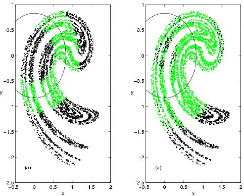
Figure 3: Consistent (grey) and inconsistent (black) predictions of the full state space Ikeda map using (a) third order truncation and (b) fifth order truncation of (4.1). The black line indicates where the truncated models are exact ($\theta=-\pi$).

It is often the case that no sufficiently relevant model equations are available and that an empirical, data-driven approach is required. There are two common strategies in this case: to construct a local model as each prediction is required or to construct a single, global model. For clarity, only local linear models and local quadratic models are employed below, while the empirical global models used are based on radial basis functions; both approaches were introduced briefly in section 3.

CND considers the local neighbourhood around the base point of the prediction. In this example, a linear model is fit to describe the evolution of historical base points within this neighbourhood towards their future images. This linear model is then applied to the base point to yield a prediction of its future image. The optimal size of the local neighbourhood ${\cal B}({\bf x},r)$, at a point ${\bf x}$ with radius $r$, depends on (i) the data density in ${\cal B}({\bf x},r)$, (ii) the magnitude of the neglected nonlinear terms in ${\cal B}({\bf x},r)$ and (iii) the measurement uncertainty of points in ${\cal B}({\bf x},r)$ (for a discussion, see [30, 31]). Local linear predictions of the noisy measurements of both $x$ and $y$ variables of the Ikeda map using $r=0.15$ and $r=0.2$ are illustrated in Fig. 4. The fraction of inconsistent predictions were $f_{inc}=0.025$ and $f_{inc}=0.27$ for $r=0.15$ and $r=0.2$ respectively. The predictor with the smaller radius of $r=0.15$ produces fewer inconsistent predictions because the local linear model is better able to capture the dynamics in this neighbourhood. This makes sense, in that for larger values of $r$ there are more locations where the local quadratic terms play a significant role and thus the linear model (which is blind to these effects) fails to yield consistent predictions.

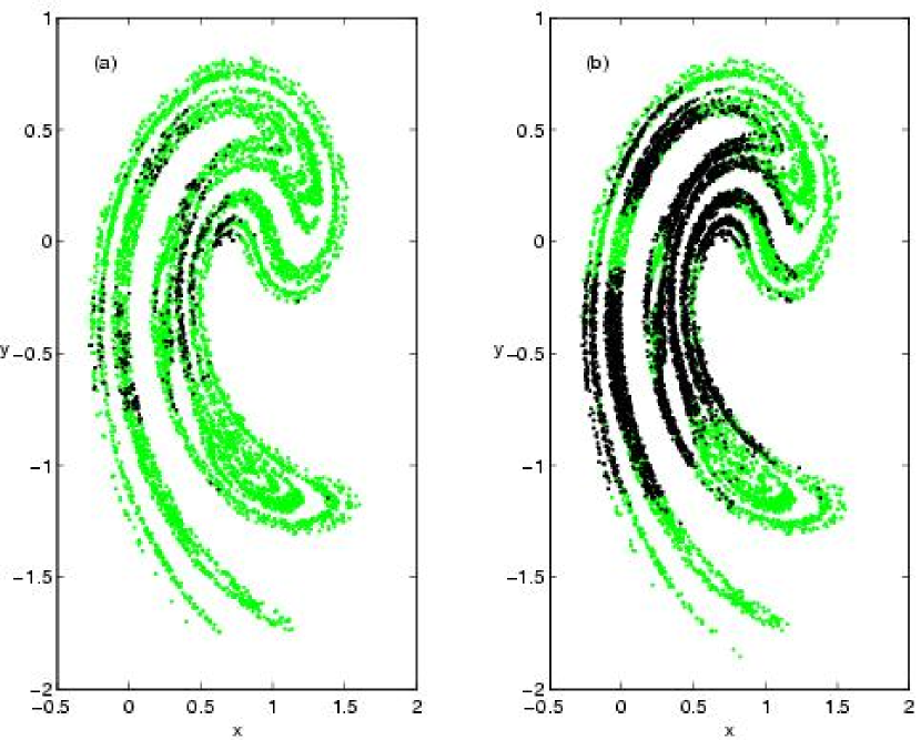
Figure 4: Consistent (grey) and inconsistent (black) predictions of the full state space Ikeda map using local linear prediction with neighbourhood radii of (a) 0.15 and (b) 0.20.

The consistency analysis can also be used to explore whether or not there are self-intersections within a reconstructed state space. For the Ikeda map, there are many self intersections using a reconstruction dimension of $m=2$ (Fig 5a). These self-intersections imply that nearby points, often called false neighbours, (Fig. 5b) will have images in different parts of the attractor (Fig 5c). The singular value decomposition of the local linear map provides a means of calculating the expected region (an ellipse under the linear approximation) where the images should fall. In this case of self-intersections, the consistency analysis correctly shows that the predictions should lie between the two extremes of the images, coloured red and blue (Fig. 5c) and the resulting inconsistent predictions reflect a failure of this reconstruction due to $m$ not being sufficiently large.

Schroer et al. [22] have shown that the fraction of the attractor which yields poor predictions due to self-intersections scales as $r^{m-D_{1}}$ where $r$ is the size of the neighbourhood used for constructing the local constant predictor and $D_{1}$ is the information dimension. A noise-free time series of the $x$-coordinate of the Ikeda map (9) significant to four decimal places was generated and used to provide a reconstructed state space with $m=2$. Local linear predictions with a neighbourhood of radius $r$ were analysed for consistency against a noise threshold of $\epsilon=5\times 10^{-5}$ using (4). The fraction of inconsistent points $f_{inc}$ decreases with the size of the local neighbourhood radius $r$ according to $f_{inc}\propto r^{m-D_{1}}$ (Fig. 6), in agreement with the theoretical calculations [22]. $D_{1}$ was estimated using the Kaplan-Yorke conjecture [32]

$$D_{1}=D_{Lyap}\equiv k+\frac{\sum_{i=1}^{k}\lambda_{i}}{\lambda_{k+1}}$$ (11)

where $D_{Lyap}$ is the Lyapunov dimension, $\lambda_{i}$ are the Lyapunov exponents and $k$ is defined such that $\sum_{i=1}^{k}\lambda_{i}\geq 0$ and $\sum_{i=1}^{k+1}\lambda_{i}<0$. For the Ikeda system with parameter values $a=0.4,b=6.0$ and $\mu=0.9$, $D_{Lyap}=1.71$ (for discussion, see McSharry [23]).

4.2 False nearest neighbours

The method of false nearest neighbours introduced by Kennel et al. (see [15] and references thereof), is commonly used to select a “sufficient” dimension for models based on a delay reconstruction; here “sufficient” means large enough to resolve the dynamics without self-intersection of likely solutions in the (projected) perfect model . Let $d_{ij}(m)$ denote the distance between two state vectors ${\bf s}_{i}$ and ${\bf s}_{j}$ in a reconstructed state space of dimension $m$. This method relies on identifying the fraction of false near neighbours, that is pairs of points whose separations $d_{ij}(m)$ and $d_{ij}(m+1)$ satisfy $\Delta({\bf s}_{i},{\bf s}_{j},m)=d_{ij}(m+1)/d_{ij}(m)>\gamma$. A shortcoming of that approach to the detection of these false near neighbours [15] is the arbitrary threshold $\gamma$ which determines which pairs are “false”. In a state space where the dimension $m$ is sufficient to remove all self-intersections $\Delta({\bf s}_{i},{\bf s}_{j},m)$ will be dependent on the structure of the dynamics in the neighbourhood of ${\bf s}_{i}$ and ${\bf s}_{j}$ and thus is expected to vary throughout the model-state space if ${\bf s}_{i}$ varies.

An alternative method for identifying a sufficient dimension $m$ is to make local linear predictions using different values of $m$. If self-intersections exist, the fraction of inconsistent points will scale as $f_{inc}=r^{m-D_{1}}$, otherwise $f_{inc}$ should drop to zero for a sufficiently small value of $r$. In any case $\gamma$ should be allowed to vary with $x$; within the local linear model, for example, it can vary with $sigma_{1}$.

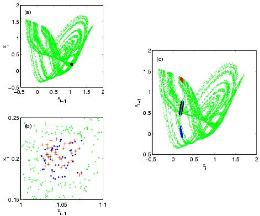
Figure 5: An illustration of self-intersection in a $m=2$ reconstruction of the Ikeda map: (a) the reconstructed state space $(x_{i-1},x_{i})$ showing observed points within a square centred at the base-point (1.05,0.2) being consistent with measurement errors of magnitude $\epsilon=0.025$, (b) a zoom-in showing pre-images of points which have large $x_{i+1}$ (pluses) and points which have small values of $x_{i+1}$ (dots) and (c) the reconstructed state space $(x_{i},x_{i+1})$ with images from (b), corresponding local linear predictions (black) and consistency ellipse (grey).

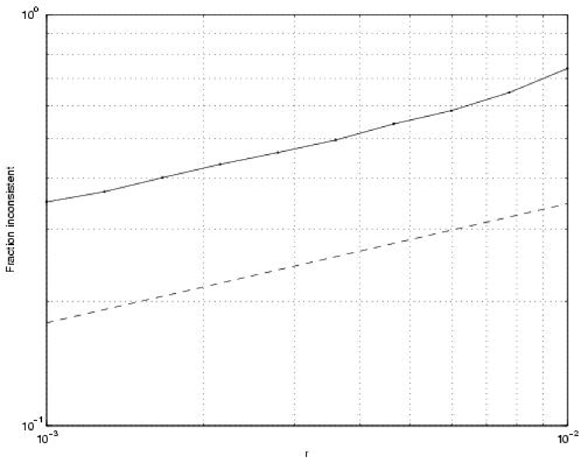
Figure 6: Fraction of inconsistent predictions as a function of the neighbourhood radius $r$ used for fitting the local linear model (solid). The dashed line indicates the theoretical slope given by $m-D_{1}=2-1.71=0.29$.

4.3 Rulkov circuit equations

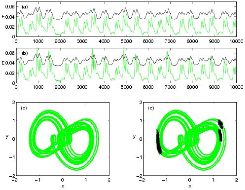
Figure 7: Consistency analysis of the Rulkov circuit. The upper panels illustrate the prediction errors for the perfect model (a) imperfect model (b). The grey line is the prediction error and the black line is the consistency envelope. Points above the envelope are inconsistent. The lower panels are 2D projections of the delay reconstruction showing both consistent points (grey dots) and inconsistent points ($\times$) for perfect (c) and imperfect model (d).

A second mathematical system will be used to illustrate how CND can identify state space dependent model error, in this case due to incorrect parameter values. The system is the set of equations defining Rulkov’s circuit [33, 34] are

$${\dot{x}} = y,$$

$${\dot{y}} = -x-\delta y+z,$$

$${\dot{z}} = \gamma\left[\alpha f(x(t))-z\right]-\sigma y,$$ (12)

where $x(t)$ is the voltage across the capacitor $C$, $y(t)=\sqrt{\frac{L}{C}}i(t)$ with $i(t)$ the current through the inductor $L$, and $z(t)$ is the voltage across the the capacitor $C^{\prime}$. Time has been scaled by $\frac{1}{\sqrt{LC}}$. The parameters of this system have the following dependence on the physical values of the circuit elements

$$\gamma=\frac{\sqrt{LC}}{RC^{\prime}},\ \delta=r\sqrt{\frac{C}{L}},\ \sigma=\frac{C}{C^{\prime}}.$$ (13)

The function $f(x)$ is

$$f(x)=\left\{\begin{array}[]{ll}0.528,&\mbox{$x\leq-x_{a}$}\\ x(1-x^{2}),&\mbox{$-x_{a}<x<x_{a}$}\\ -0.528,&\mbox{$x\geq x_{a}$}\end{array}\right.,$$ (14)

and the control parameter $\alpha$ characterises the gain of the nonlinear amplifier around $x=0$. The parameters of the circuit correspond to the following values for the coefficients in the differential equations (12): $\gamma=0.294$, $\sigma=1.52$, $\delta=0.534$, $\alpha=15.6$ and $x_{a}=1.2$.

The model is the same set of equations but with $x_{a}=1.4$, thus the model is structurally correct, has one parameter in error; all other parameters are exactly the same as the system.

CND is now used to map out regions of inconsistent points in the state space. The observations consist of three dimensional time series of $x$, $y$ and $z$ variables, forming a state vector ${\bf x}=(x,y,z)$, contaminated with additive measurement noise independently and uniformly distributed on $[-\epsilon,\epsilon]$; $\epsilon=0.01$. Numerical integration of (12) using a fourth order Runge-Kutta method [26] with a fixed integration step yields a discrete-time map. Given an observed initial condition ${\bf x}_{0}={\bf x}(t_{0})$ and an initial uncertainty $\mbox{\boldmath${\epsilon}$}(t_{0})$ at time $t_{0}$, the uncertainty after an arbitrary time $\tau$ is

$$\mbox{\boldmath${\epsilon}$}(t_{0}+\tau)=\mbox{\boldmath${{\cal M}}$}({\bf x}_{0},\tau)\mbox{\boldmath${\epsilon}$}(t_{0}),$$ (15)

where the matrix ${\mbox{\boldmath${\cal M}$}}({\bf x}_{0},\tau)$ is the linear propagator defined by

$$\mbox{\boldmath${{\cal M}}$}({\bf x}_{0},\tau)=\exp\left[\int_{t_{0}}^{t_{0}+\tau}\mbox{\boldmath${\cal J}$}{\bf(}{\bf x}(t){\bf)}dt\right],$$ (16)

and $\mbox{\boldmath${\cal J}$}{\bf(}{\bf x}(t){\bf)}$ is the Jacobian of the flow given by (12). Taking discrete steps of size $\tau=0.01$, the model was then used to provide one step ahead predictions of the values of the three-dimensional state vector ${\bf x}=(x,y,z)$.

CND analysis of a model with $x_{a}=1.4$ can be contrasted with that of a perfect model (that is, $x_{a}=1.2$) to demonstrate how the approach identifies regions of model-state space with systematic errors due to parameter uncertainty.

The first singular value of the linear propagator ${\mbox{\boldmath${\cal M}$}}({\bf x}_{0},\tau)$ provides a consistency bound (4) for each prediction (Fig. 7). As expected, the perfect model with $x_{a}=1.2$ yields no inconsistent points (Fig. 7a and 7c) whereas the model with $x_{a}=1.4$ gives rise to occasional inconsistent predictions (Fig. 7b and 7d), the location of which correctly diagnoses the (known) model imperfection. In this way, a CND analysis can be used to identify “synoptic patterns” where models tend to fail. This identification does not replace the need for insight and physical understanding to determine how to improve the model, rather CND merely identifies where the model is most vulnerable; and it can be applied to the largest of numerical simulation models.

5 Forecasting physical systems

In this section CND is applied to three physical systems; in each case the performance of previously published models are contrasted. While the state space reconstructions appear adequate to resolve the dynamics, these examples demonstrate that other problems arise which are model dependent. The local linear is inaccurate when nonlinear terms dominate in the local neighbourhood to collect sufficient near neighbours to estimate the model parameters. This problem often arises when some regions of the state space are sparsely sampled, thereby requiring a large neighbourhood. The RBF model provides a global approximation to the dynamics, but is likely to yield a good fit of regions of state space with a high data density while neglecting those which are poorly sampled [14]. CND provides a means of identifying and addressing all these problems and suggests a method for selectively using different models with complementary strengths and weaknesses.

5.1 Power output from NH₃ laser

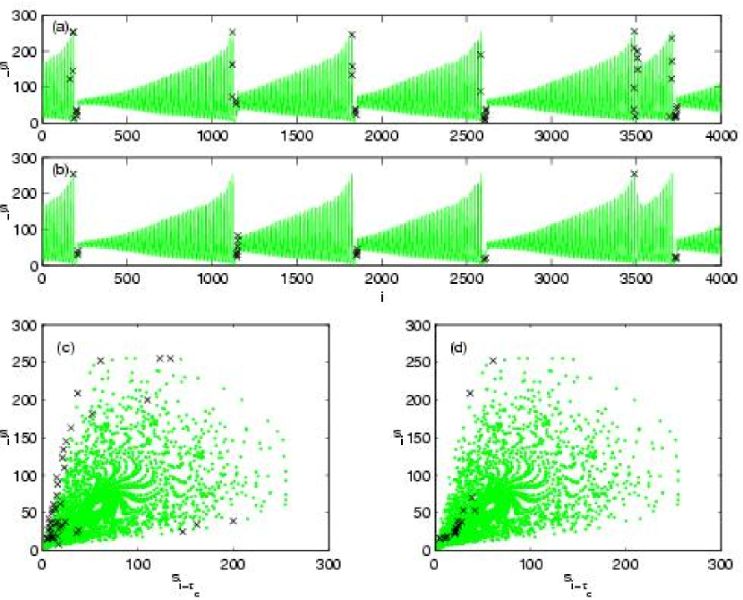
Figure 8: Predictions of the NH₃ laser data. The upper panels illustrate the inconsistent predictions ($\times$) for models RBF₁ (a) and LL_1a (b). The lower panels are 2D projections of the delay reconstruction showing both consistent points (grey dots) and inconsistent points ($\times$) for RBF₁ (c) and LL_1a (d).

Fig. 8a shows the output power of a ${\rm NH}_{3}$ laser whose dynamics are associated with the Lorenz-Haken equations [35]; this dataset, collected by Hüner et al. [36], has been widely studied (see Weigend and Gershenfeld [37], and references thereof). The noise level is taken to be below the resolution of an (8 bit) analogue to digital converter, thus $\epsilon=1$. Following Smith [38], a Local Linear model (LL_1a), was employed to make one-step predictions and compared with a Radial Basis Function model (RBF₁). Both models use the same delay reconstruction parameters (see Table 1). Typical segments of the time series and images of inconsistent predictions are plotted for both models in Fig. 8. Note that all the inconsistent points occur around the collapses; this may result either from the relatively sparse sampling of this region of model-state space or a local failure of the embedding [38]. A 2D projection of the 4D reconstructed model-state space is illustrated in Fig. 8c and 8d, showing the origins of the inconsistent predictions for each model. If the reconstruction parameters, $m$ and $\tau_{d}$ are sufficient to resolve the dynamics, it may be possible to improve the consistency by employing a neighbourhood size which is suitable for the local linear approximation [30].

The problem of low data density around the collapses was addressed by using a different LL model (LL_1b) with a smaller neighbourhood size given by $k=8$, thereby preventing neighbours with different dynamics from heavily influencing the predictions in data sparse regions. This new LL model removes some inconsistent predictions at the beginning of the collapses, but adds some new inconsistent predictions at the end of the collapses (Fig. 8d and stars in 9b).

The fact that some predictions are inconsistent for one model, yet consistent for another (Fig. 9) suggests that a hybrid predictor using both of these models selectively would outperform any one individual model; indeed such a hybrid model for this system is presented by Smith [38] based on RMS error criteria. One advantage of using a CND criteria instead is that it focuses attention on regions of model inadequacy, even when the one-step RMS error may be rather small. RBF predictions with large absolute errors tend to correspond with small LL_1b errors and vice versa (Fig. 9). While the RBF has inconsistent predictions at the beginning of the collapses, LL_1b gives inconsistent predictions at the end of the collapse, just as the intensity starts to increase again. Table 1 provides a description of the models and their prediction results and Table 2 gives a comparison of the different models. In particular, while the RBF and LL_1b models generate 1.13% and 0.48% inconsistent predictions individually, they have only 0.1% in common. Furthermore LL_1b provides a better complement to RBF than LL_1a since there are 0.15% inconsistent predictions shared between RBF and LL_1a.

To establish whether or not an in-sample CND analysis of the learning set might contain information on out-of-sample forecasts, a hybrid model was constructed. Following Smith [14, 30], the RBF centres were used to define a Voronoi partition of the state space and the fraction $p_{j}$ of inconsistent predictions in each partition $j$ ($j=1,\ldots,N_{c})$ was calculated by making in-sample predictions of the learning data set. For each base point ${\bf s}_{i}$ belonging to a partition which had one or more in-sample inconsistent predictions, a local linear model (either LL_1a or LL_1b) was used to generate a prediction. If the inconsistent regions of state space are clustered in state space and the local linear models are complementary to the RBF model, then this hybrid should improve the prediction performance. Indeed, both the combined models, RBF₁LL_1a and RBF₁LL_1b had smaller RMS errors than their constituent models and also lower fractions of inconsistent predictions (Table 1).

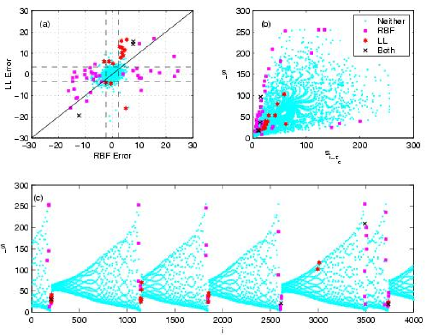
Figure 9: Consistency analysis of the NH₃ laser data showing (a) prediction errors for the RBF₁ and LL_1b models, (b) 2D projections of the delay reconstruction and (c) the time series. Markers indicate one of four outcomes: (i) neither model is inconsistent (dot), (ii) RBF₁ is inconsistent (square), (iii) LL_1b is inconsistent (hexagon) or (iv) both models are inconsistent (cross). Dashed lines reflect plus and minus one standard deviation of the error distribution for each model in (a).

5.2 Power output from an NMR laser

Figure 10: Predictions of the NMR laser data contrasting models RBF₂ and LL_2a. The upper panels illustrate the inconsistent predictions ($\times$) for models RBF₂ (a) and LL_2a (b). The lower panels are 2D projections of the delay reconstruction showing both consistent points (grey dots) and inconsistent points ($\times$) for RBF₂ (c) and LL_2a (d).

Figure 10a illustrates a stroboscopic view of the output power of a nuclear magnetic resonance (NMR) laser operated at ETH Zürich [39]. The lasing particles are Al atoms in a ruby crystal, and the quality factor of the resonant structure is modulated periodically. Output power of the laser is reflected in the voltage across the antenna (thus allowing for negative values). A local linear model (LL_2a) and a RBF model (RBF₂) were constructed following Kantz and Schreiber [9]. Details of the models are given in Table 1. The model LL_2a had a fixed radius neighbourhood of size $r=50$ (allowing the number of neighbours to vary); this is roughly equal to twice the amplitude of the reported measurement error amplitude, $\epsilon=25$. Inconsistent points are shown in Fig. 10a and 10c for the RBF model and in Fig. 10b and 10d for the LL_2a model. The inconsistent predictions typically originate from the same location of model-state space. In this case, reconstructed vectors from regions where a large positive observation follows a large negative observation tended to be inconsistent.

This insight from the CND analysis suggests examining the scatter plot of the prediction errors (Fig. 11a). This figure shows that errors generated by the RBF and LL_2a models are highly correlated, with both making errors of similar sign and magnitude. By zooming into the inconsistent region of the attractor, it becomes clear that model inadequacy around the elbow of the attractor, shown for the base of the inconsistent points (Fig. 11b) and their images (Fig. 11c), causes both models to fail. This effect is most noticeable for the LL_2a model at the elbows of the attractor. In contrast, the ability of the LL_2a model to resolve dynamics in a small neighbourhood provides consistent predictions in the upper part of the attractor (Fig. 11b) whereas the RBF model is unable to resolve the dynamics around the two leaves of the attractor.

One method for addressing the failure of the LL_2a model to approximate the dynamics at the elbow of the attractor (Fig. 11b) is to use a local quadratic (LQ) model. A LQ model (LQ_2a) with neighbourhood $r=50$ did not change the number of inconsistent predictions and increased the prediction errors (Table 1). By decreasing the radius to $r=25$, a new LQ model (LQ_2b) decreased the fraction of inconsistent predictions (from 1.4% to 0.5%) at the elbow at the expense of increasing the overall prediction accuracy (Table 1).

The benefit of using two models together may be seen from the fractions of inconsistent predictions in the different scenarios (Table 2). While the RBF and LQ_2b independently have 1.65% and 0.83% inconsistent predictions respectively (Table 1), they only have 0.375% inconsistent predictions in common. Note that the local models using large neighbourhoods, LL_2a and LQ_2a, offer little compensation to the model inadequacy in the RBF model.

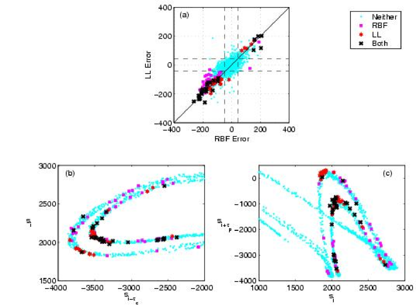
Figure 11: Consistency analysis of the NMR laser data showing (a) prediction errors for the models RBF₂ and LL_2a models, (b) return map of $s_{i}$ versus $s_{i-\tau_{d}}$ and (c) return map of $s_{i+\tau_{p}}$ versus $s_{i}$. Markers indicate one of four outcomes: (i) neither model is inconsistent (dot), (ii) RBF is inconsistent (square), (iii) LL_2a is inconsistent (hexagon) or (iv) both models are inconsistent (cross).

An alternative to changing the structure of the model is simply to alter the local neighbourhood size; this can even lead to a meaningful reduction of the RMS error. This is illustrated in the next paragraph by taking the inconsistent points of model (LL_2a) and predicting them with a LL model (LL_2b) that uses a fixed number of neighbours given by $k=12$. While LL_2b has a slightly higher RMS error than LL_2a, it reduces the fraction of inconsistent predictions from 1.4 to 0.5 (Table 1).

As noted in the introduction, the appropriateness of each local linear model can be determined by examining the expected value of the observational noise divided by the (local) length scale at which quadratic (higher order) terms become important. CND can suggest where in the model-state space this fundamental ratio is large, and in such locations one must consider local quadratic models as above. In regions where this ratio is small, and the length scale at which quadratic terms become important is also small, it is advantageous to take smaller neighbourhoods thereby improving the local linear model. In this case CND successfully identifies such regions. Figure 12a shows the expected magnification in a LL_2b model plotted against the that of the LL_2a model for only those points where the LL_2a model is not consistent. The fact that the points generally lie above the diagonal indicates that the LL_2b model is (locally) more sensitive to uncertainty than the LL_1a model which averages effects over a larger area. Not only does this increased sensitivity correctly reduce inconsistency, it also leads to better (local) predictions, as indicated by Fig. 12b, the corresponding scatter diagram of observed prediction error. For these points the LL_2b model has a lower median error, lower RMS error, and predicts 66% of the points more accurately.

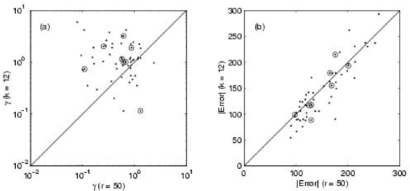
Figure 12: A comparison between models LL_2a ($r=50$) and LL_2b ($k=12$) for predictions which are inconsistent under LL_2a: (a) magnification factors $\gamma$ and (b) absolute prediction errors. Circles indicate points that are also inconsistent in LL_2b.

5.3 Temperature data from a Fluid Annulus

Figure 13a shows a time series from a temperature probe in a rotating annulus of fluid [40, 41]. A classic experiment in geophysics which Lorenz [42] cited as physical motivation for deterministic aperiodic flow, the annulus consists of thermally conducting side walls and insulating boundaries on the top and bottom. A temperature difference is maintained between the inner and outer side walls, providing an infinite dimensional simulation of the mid-latitude circulation of the Earth’s atmosphere. Following [14], one step ahead predictions were made using a local linear model (LL₃) and a RBF model (RBF₃). See Table 1 for details of the models. The data was assumed to have uniformly distributed noise of amplitude $\epsilon=0.1$. The inconsistent points (Fig. 13) reveal that the LL model is extremely good ($f_{inc}=0.68\%$) whereas the RBF model ($f_{inc}=2.25\%$) yields a much larger number of inconsistent predictions.

One approach for improving the consistency of the RBF model is to force it to provide a better fit to the dynamics in regions of state space which were inconsistent in the learning data set. The RBF centres were used to form a Voronoi partition of the state space and the fraction $p_{j}$ of inconsistent predictions in each partition $j$ ($j=1,\ldots,N_{c})$ was calculated using in-sample predictions of points in the learning data set. Following Smith [14] which re-weighted partitions to get a more uniform error in the model-state space, CND analysis provides the information required to construct an RBF model which better approximates the more inconsistent partitions (those with large values of $p_{j}$). This is done by providing weights ${\bf w}=\{w_{i}\}_{i=1}^{N_{l}}$ such that $w_{i}=1+\alpha p_{n(i)}$ where $n(i)$ is the index of the partition containing ${\bf s}_{i}$, and computing new parameters ${\bf a}=({\bf w}\mbox{\boldmath${\Phi}$})^{\dagger}({\bf w}{\bf b})$. This new weighted RBF (hereafter, WRBF) model will have a higher RMS error since, by definition, the RMS error is minimised when $w_{i}=1$ for all $i$. While the prediction errors will increase in the partitions with small $p_{j}$, the WRBF can be used to reduce the overall number of inconsistent predictions. The value of $\alpha$ controls the balance between increasing the RMS error and improving the consistency. Using $\alpha=128$, the fraction of inconsistent predictions was decreased, from $2.25\%$ for the RBF model to $1.07\%$ for the WRBF model, whereas the RMS (normalised by the standard deviation of the data) increased from 0.47 to 0.89. Many of the large RBF errors were improved by the WRBF (Fig. 14a) yielding less inconsistent predictions (Fig. 14b and 14c). The fraction of inconsistent predictions shared by the RBF and WRBF is only 0.586% (Table 2). This small fraction is equal to the fraction of shared inconsistent predictions for the RBF and the LL. While it is to be expected that the RBF and LL would yield different inconsistent predictions because of the disparity between their model structures, this result suggests that the weights provide a means of obtaining a complementary version of a given RBF model.

A hybrid model RBFWRBF was constructed using the RBF to make predictions in all partitions except those where there were one or more inconsistent predictions in the learning set. In this case the inconsistent predictions are not clustered and so the hybrid gives a medium level of performance, having a lower RMS error than the WRBF but a higher RMS error than the RBF.

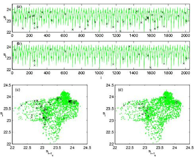
Figure 13: Predictions of the Annulus data contrasting models RBF₃ and LL₃. The upper panels illustrate the inconsistent predictions ($\times$) for models RBF₃ (a) and LL₃ (b). The lower panels are 2D projections of the delay reconstruction showing both consistent points (grey dots) and inconsistent points ($\times$) for RBF₃ (c) and LL₃ (d).

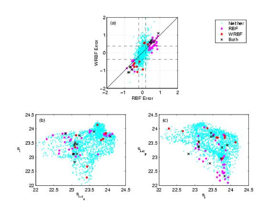
Figure 14: Consistency analysis of the Annulus data contrasting models RBF and WRBF: (a) prediction errors for the models RBF₃ and WRBF, (b) return map of $s_{i}$ versus $s_{i-\tau_{d}}$ and (c) return map of $s_{i+\tau_{p}}$ versus $s_{i}$. Markers indicate one of four outcomes: (i) neither model is inconsistent (dot), (ii) RBF₃ is inconsistent (square), (iii) WRBF is inconsistent (star) or (iv) both models are inconsistent (cross).

6 Discussion

A new test for Consistent Nonlinear Dynamics (CND) has been introduced and illustrated on a number of examples. The key aim of CND is to quantify the consistency between a model’s dynamics and the observations locally throughout the model-state space. Regions of systematic failure indicate states of the system where the model needs improvement, regardless of whether the absolute value of the errors in that region are large or small. Similarly, regions of large errors which are consistent with the model dynamics and level of observational uncertainty should not be counted against the model a priori. In such regions the observations are consistent with the model forecasts, and the model can be accepted. Of course, this acceptance is provisional, the model may well fail to remain consistent when the noise level is reduced, or another (locally) consistent model may be found to have better error statistics in this region and longer shadowing times. In any event, lower one-step forecast errors per se need not indicate a better model. The errors of the best first guess forecast are simply beside the point: the simplest model consistent with the data should admit trajectories consistent with the observations.

Where the model has been consistent, prognostic assessment of the likely accuracy of predictions can be made in real-time, while in regions of the model state space where the model tends to be inconsistent model based estimates of predictability (whether analytic, or made with ensemble forecasts [7]) should not be relied upon; in such regions historical errors may prove to be of value [14].

Other insights from the application of CND include:

(i) The distribution of prediction errors from a nonlinear model is expected to show correlation in state space and thus show significant residual predictability [30, 3]. Equation (2) shows that this is to be expected even with a perfect nonlinear model: the local residuals need not be symmetrically distributed about the global mean error [3, 23].

(ii) The original method of false nearest neighbours [15] can be strengthened, replacing the arbitrary global threshold used to define “false” by adopting a local threshold based on the internal consistency of the dynamics.

(iii) Noise reduction strategies often use a variational approach [7]; the interpretation of a variational data assimilation scheme assumes the existence of a consistent model trajectory. CND can verify this assumption.

(iv) The ‘optimal linear predictor’ is often inconsistent with the observations in a systematic manner; CND will detect this.

(v) All models of physical systems contain structural error; no single best model need exist (for discussion, see [5, 43, 44]). Rather than trying to obtain a single optimal model, it may be prove effective to consider ensembles over models with different model structures. Ensembles over different initial conditions are often utilised to account for observational uncertainty [4, 5, 7]. Results from this paper suggest a complementary method which accounts for structural uncertainty by employing ensembles over model structures (see [23, 43]).

(vi) Systematic changes in the frequency or location of inconsistent points may indicate non-stationarity in the underlying process [14].

(vii) Given a data stream, selective refinement of points corresponding to inconsistent regions is expected to yield a better data base for local models than uniform sampling, at least in the noise-free case for local polynomial models [30, 23, 45].

Table 1: Description of the models used for the three physical systems. Reconstruction parameters are dimension $m$, time delay $\tau_{d}$, and dataset sizes used for learning $N_{l}$, and testing $N_{t}$ (in 1000s). $N_{c}$ is the number of RBF centres and $\phi(r)$ gives the structure of the RBF. The LL neighbourhood is defined by the number of neighbours $k$ or the radius $r$. Error is the RMS forecast error normalised by the standard deviation of the data and $\%f_{inc}$ is the percentage of inconsistent predictions.

Key	System	$m$	$\tau_{d}$	$\tau_{p}$	$N_{l}$	$N_{t}$	$N_{c}$	$\phi(r)$	$k$	$r$	Error	$\%f_{inc}$
RBF1	NH3	4	2	1	21	4	128	$r^{3}$			0.0514	1.13
LL1a	NH3	4	2	1	21	4			32		0.0381	0.53
LL1b	NH3	4	2	1	21	4			8		0.0797	0.48
RBF1LL1a	NH3	4	2	1	21	4	128	$r^{3}$	32		0.0376	0.30
RBF1LL1b	NH3	4	2	1	21	4	128	$r^{3}$	8		0.0451	0.27
RBF2	NMR	3	1	1	30	4	128	$r^{3}$			0.0207	1.65
LL2a	NMR	3	1	1	30	4				50	0.0189	1.40
LL2b	NMR	3	1	1	30	4			12		0.0197	0.50
LQ2a	NMR	3	1	1	30	4				50	0.0210	1.40
LQ2b	NMR	3	1	1	30	4				25	0.0243	0.83
RBF3	Annulus	5	4	18	2	4	128	$e^{-r^{2}/2\sigma_{2}}$			0.4764	2.25
LL3	Annulus	5	4	18	2	2			32		0.4207	0.68
WRBF	Annulus	5	4	18	2	2	128	$e^{-r^{2}/2\sigma_{2}}$			0.8989	1.07
RBFWRBF	Annulus	5	4	18	2	2	128	$e^{-r^{2}/2\sigma_{2}}$			0.5402	1.27

Table 2: Comparison between two models A and B. Percentage of predictions falling into each of four scenarios: (i) Neither A nor B are inconsistent, (ii) only A is inconsistent, (iii) only B is inconsistent and (iv) both A and B are inconsistent.

System	Model A	Model B	(i)	(ii)	(iii)	(iv)
NH3	RBF1	LL1a	98.500	0.975	0.375	0.150
NH3	RBF1	LL1b	98.500	1.025	0.375	0.100
NMR	RBF2	LL2a	97.675	0.925	0.700	0.700
NMR	RBF2	LL2b	98.000	1.500	0.375	0.125
NMR	RBF2	LQ2a	97.600	1.000	0.775	0.625
NMR	RBF2	LQ2b	97.925	1.250	0.450	0.375
NMR	LL2a	LL2b	98.300	1.200	0.300	0.200
Annulus	RBF3	LL3	97.656	1.660	0.098	0.586
Annulus	RBF3	WRBF	97.266	1.660	0.489	0.586

7 Conclusion

A new approach for finding the limitations of dynamical models has been proposed and illustrated. By examining the consistency of the local model dynamics with the observed system dynamics, the consistent nonlinear dynamics (CND) approach can identify regions of the model-state space where the model is systematically inconsistent. Analysis of two theoretical systems and three physical systems illustrates that this novel consistency test contains a wealth of information about a model’s ability to approximate the observed dynamics in general, and delay reconstructions in particular. If the delay reconstruction does not yield an embedding, then all models will be inconsistent in regions where the embedding fails. When an embedding does exist, distinct model structures may be preferred in certain regions; CND identifies these explicitly. Each analysis yields a direct assessment of individual predictions, taking the local properties of the model structure into account, thereby avoiding biases arising from model sensitivity.

Uncovering the failure or success of candidate model structures provides a useful discriminator for contrasting different models. The ultimate aim here is to find better models, and a better way to define ”better” in this context. Locally consistent models are expected to allow longer shadowing trajectories; a comparison along these lines will be presented elsewhere.

By adopting CND as a goal, one aims to get the simplest models consistent with the data, but none simpler. RMS skill scores can prove a distraction in this quest. By addressing the interplay between the nonlinear model structure and observational uncertainty in the measurement process, the CND approach opens many avenues for both the evaluation and the application of nonlinear models.

References

- [1] R. P. Feynman. The Character of Physical Law. Penguin Books, London, 1992.
- [2] C. Chatfield. The Analysis of Time Series. Chapman and Hall, London, New York, 4th edition, 1989.
- [3] P. E. McSharry and L. A. Smith. Better nonlinear models from noisy data: Attractors with maximum likelihood. Phys. Rev. Lett., 83(21):4285–4288, 1999.
- [4] L. A. Smith. The maintenance of uncertainty. In G. Cini, editor, Nonlinearity in Geophysics and Astrophysics, volume CXXXIII of International School of Physics “Enrico Fermi”, pages 177–246, Bologna, Italy, 1997. Società Italiana di Fisica.
- [5] L. A. Smith. Disentangling uncertainty and error: On the predictability of nonlinear systems. In A. I. Mees, editor, Nonlinear Dynamics and Statistics, pages 31–64, Boston, 2000. Birkhauser.
- [6] C. Grebogi, S. M. Hammel, J. A. Yorke, and T. Sauer. Shadowing of physical trajectories in chaotic dynamics: Containment and refinement. Phys. Rev. Lett., 65:1527–1530, 1990.
- [7] T. N. Palmer. Predicting uncertainty in forecasts of weather and climate. Rep. Prog. Phys., 63:71–116, 2000.
- [8] D. Orrell, L. A. Smith, J. Barkmeijer, and T. N. Palmer. Model error in weather forecasting. Nonlinear Processes in Geophysics, 8(6):357–371, November 2001.
- [9] H. Kantz and T. Schreiber. Nonlinear Time Series Analysis. Cambridge University Press, Cambridge, 1997.
- [10] J. D. Farmer and J. J. Sidorowich. Predicting chaotic time series. Phys. Rev. Lett., 59(8):845–848, 1987.
- [11] M. B. Priestly. Spectral Analysis and Time Series. Academic Press, London, 1981.
- [12] D. S. Broomhead and D. Lowe. Multivariable functional interpolation and adaptive networks. J. Complex Systems, 2:321–355, 1988.
- [13] M. Casdagli. Nonlinear prediction of chaotic time series. Physica D, 35:335–356, 1989.
- [14] L. A. Smith. Identification and prediction of low-dimensional dynamics. Physica D, 58:50–76, 1992.
- [15] M. B. Kennel, R. Brown, and H. D. I. Abarbanel. Determining embedding dimension for the phase-space reconstruction using a geometrical construction. Phys. Rev. A, 45(6):3403–3411, 1992.
- [16] H. Tong. Non-Linear Time Series Analysis. Oxford Univ. Press, Oxford, 1990.
- [17] E. J. Kostelich and J. A. Yorke. Noise-reduction – finding the simplest dynamic system consistent with the data. Physica D, 41(2):183–196, 1990.
- [18] K. Judd and L. A. Smith. Indistinguishable states II: imperfect model scenario. Physica D, 2004. in review.
- [19] K. J. Beven. Equifinality, data assimilation, and uncertainty estimation in mechanistic modelling of complex environmental systems. J. Hydrology, 249:11–29, 2001.
- [20] K. J. Beven. Towards a coherent philosophy for modelling the environment. Proc. Roy. Soc. A, 458:2465–2484, 2002.
- [21] D. Orrell. Modelling nonlinear dynamical systems: chaos, uncertainty, and error. PhD thesis, University of Oxford, 2001.
- [22] C. G. Schroer, T. Sauer, E. Ott, and J. A. Yorke. Predicting chaos most of the time from embeddings with self-intersections. Phys. Rev. Lett., 80(7):1410–1413, 1998.
- [23] P. E. McSharry. Innovations in Consistent Nonlinear Deterministic Prediction. PhD thesis, University of Oxford, 1999.
- [24] F. Takens. Detecting strange attractors in fluid turbulence. In D. Rand and L. S. Young, editors, Dynamical Systems and Turbulence, volume 898, page 366, New York, 1981. Springer-Verlag.
- [25] T. Sauer, J. A. Yorke, and M. Casdagli. Embedology. J. Stats. Phys., 65:579–616, 1991.
- [26] W. H. Press, B. P. Flannery, S. A. Teukolsky, and W. T. Vetterling. Numerical Recipes in C. CUP, Cambridge, 2nd edition, 1992.
- [27] K. Ikeda. Multiple-valued stationary state and its instability of the transmitted light by a ring cavity system. Optics Communications, 30(2):257–261, 1979.
- [28] K. Ikeda and H. Daido. Optical turbulence: chaotic behaviour of transmitted light from a ring cavity. Phys. Rev. Lett., 45(9):709–712, 1980.
- [29] S. M. Hammel, C. K. R. T. Jones, and J. V. Moloney. Global dynamical behaviour of the optical field in a ring cavity. J. Opt. Soc. Am. B, 2(4):552–564, April 1985.
- [30] L. A. Smith. Local optimal prediction: Exploiting strangeness and the variation of sensitivity to initial condition. Phil Trans R Soc Lond A, 348(1688):371–381, 1994.
- [31] E. M. Bollt. Model selection, confidence, and scaling in predicting chaotic time-series. Int. J. Bif. Chaos, 10(6):1407–1422, 2000.
- [32] J. L. Kaplan and J. A. Yorke. Chaotic behaviour of multidimensional difference equations. In H. O. Peitgen and H. O. Walter, editors, Functional Differential Equations and Approximation of Fixed Points, volume 730 of Lecture Notes in Mathematics, page 204. Springer, Berlin, 1979.
- [33] N. F. Rulkov, L.S. Tsimring, and H. D. I. Abarbanel. Tracking unstable orbits in chaos using dissipative feedback control. Phys. Rev. E, 50(1):314–324, 1994.
- [34] J. Timmer, H. Rust, W. Horbelt, and H. U. Voss. Parametric, nonparametric and parametric modelling of a chaotic circuit time series. Physics Letters A, 274:123–134, 2000.
- [35] H. Haken. Analogy between higher instabilities in fluids and lasers. Phys. Lett. A, 53:77, 1975.
- [36] U. Hübner, C. O. Weiss, N. B. Abraham, and D. Tsang. Lorenz-like chaos in -fir lasers. In A. Weigend and N. Gershenfeld, editors, Time Series Prediction: Forecasting the Future and Understanding the Past, volume XV of SFI Studies in Complexity, pages 323–344, New York, 1993. Addison-Wesley.
- [37] A. S. Weigend and N. A. Gershenfeld. Time Series Prediction: Forecasting the Future and Understanding the Past, volume XV of SFI Studies in Complexity. Addison-Wesley, New York, 1993.
- [38] L. A. Smith. Does a meeting in Santa Fe imply chaos? In A. Weigend and N. Gershenfeld, editors, Time Series Prediction: Forecasting the Future and Understanding the Past, volume XV of SFI Studies in Complexity, pages 323–344, New York, 1993. Addison-Wesley.
- [39] L. Flepp, R. Holzner, E. Brun, M. Finardi, and R. Badii. Model identification by periodic-orbit analysis for NMR-laser chaos. Phys. Rev. Lett., 67:2244–2247, 1991.
- [40] P. L. Read. Applications of singular systems to ‘baroclinic chaos’. Physica D, 58:455–468, 1992.
- [41] R. Hide. An experimental study of thermal convection in a rotating liquid. Phil. Trans. Roy. Soc. A, 250:441–478, 1958.
- [42] E. N. Lorenz. Deterministic nonperiodic flow. J. Atmos. Sci., 20:130–141, 1963.
- [43] L. A. Smith. Predictability past predictability present. In Seminar on predictability, pages 219–242, ECMWF, Reading, UK, 2003.
- [44] P. E. Rapp, T. I. Schmah, and A. I. Mees. Models of knowing and the investigation of dynamical systems. Physica D, 132:133–149, 1999.
- [45] F. Kwasniok and L. A. Smith. Real-time construction of optimized predictors from data streams, 2004. accepted.