Stages of Relaxation of Patterns and the Role of Stochasticity on the Final Stage

Abstract

The disorder function formalism [Gunaratne et.al., Phys. Rev. E, 57, 5146 (1998)] is used to show that pattern relaxation in an experiment on a vibrated layer of brass beads occurs in three distinct stages. During stage I, all lengthscales associated with moments of the disorder grow at a single universal rate, given by $L(t)\sim t^{0.5}$. In stage II, pattern evolution is non-universal and includes a range of growth indices. Relaxation in the final stage is characterized by a single, non-universal index. We use analysis of patterns from the Swift-Hohenberg equation to argue that mechanisms that underlie the observed pattern evolution are linear spatio-temporal dynamics (stage I), non-linear saturation (stage II), and stochasticity (stage III).

I Introduction

Analysis of structures far from equilibrium and their evolution has necessitated the development and implementation of several new techniques croAhoh . The underlying physical systems are dissipative and typically exhibit sensitive dependence on initial states egoAgre ; i.e., differences between nearly identical patterns increase in time. Further, although structures formed from distinct initial states differ in detail, they appear to share features that depend only on control parameters of the physical system. These observations led Prigogine and collaborators to propose the use of irreversible statistical analysis using ensembles of solutions of a system petApri1 ; petApri2 ; hasAsap ; antAtas . However, it is a non-trivial task to identify measures appropriate to analyze a given class of structures.

We consider properties of large aspect ratio patterns that are formed via spontaneous symmetry breaking from a noisy, but otherwise structureless initial state. Patterns are generated when an external control parameter crosses a threshold, initiating a local bifurcation to a periodic array; these arrays are typically, striped, square, triangular or hexagonal croAhoh . However, due to translational and rotational invariances of the underlying system, the location and orientation of these local patches are not synchronized over the entire domain. As they grow, these patches compete with each other to produce complex patterns seen in experimental and model systems ouyAswi ; heuAgol ; bodAdeb ; rose ; melAumb ; best ; eldAvin , see Figures 1, 6 and 9. These structures, whose details are sensitively dependent on the initial state, can be considered to belong to the ensemble of patterns.

Assume that such a spatio-temporal pattern can be represented by a scalar field $u({\bf x},t)$. Several functionals of $u({\bf x},t)$ have been proposed as measures to be used in statistical descriptions. Most of these are modeled on related quantities from equilibrium statistical mechanics. The width of the structure factor $S(t)$ schAall ; eldAvin ; croAmei (i.e., the width of the peak in the azimuthal average of $\langle\hat{u}({\bf k},t)\hat{u}(-{\bf k},t)\rangle)$ is one of the more frequently studied examples. It has been shown that the evolution of a pattern from a noisy initial state consists of two distinct stages schAall : $S(t)\sim t^{-\frac{1}{2}}$ is obeyed until the peak amplitude of the field $u({\bf x},t)$ saturates, beyond which time the pattern coarsens and the decay becomes slower. For the Swift-Hohenberg equation, Elder et al. eldAvin , Cross and Meiron croAmei , and Hou et al. houAsas found that during this second stage $S(t)$ decreased as $t^{-0.20}$ when the dynamics was noise free and at a faster rate $t^{-0.25}$ otherwise. Additional quantities have been introduced to describe the second relaxation region. Hou et al. houAsas measured cumulative domain wall length as a function of time. For noise-free (resp. noisy) dynamics, it was shown to decay as $t^{-0.25}$ (resp. $t^{-0.30}$). Cross et al. croAmei showed that a stripe orientation correlation field decayed as $t^{-0.24}$.

Notice that in the second relaxation stage, distinct measures (which probe multiple features of a pattern) decay at different rates. A systematic way to study such variations is to define a field to quantify the “local” disorder, and to use multiple moments of this field to construct a family of characteristics to describe the dynamics of various lengthscales associated with the pattern ruel . Such a class appropriate for labyrinthine patterns, referred to as the disorder function, has been introduced gunAjon ; gunArat . It is defined as

$$\delta(\beta,t)=\left[\frac{(2-\beta)}{({\int d^{2}x})}\frac{\int d^{2}x|(\triangle+k^{2})u({\bf x},t)|^{\beta}}{\langle|u({\bf x},t)|\rangle^{\beta}}\right]{\bigg{/}}k^{2\beta},$$ (1)

where $k_{0}$ is the wavevector associated with the local planform, $\langle|u({\bf x},t)|\rangle$ denotes the mean of $|u({\bf x},t)|$, ${\int d^{2}x}$ is the area of the pattern, and $\delta(\beta,t)$ ($0\leq\beta<2$) has been normalized to be scale invariant. In this definition, the field used to quantify the local disorder is the magnitude $|(\triangle+k^{2})u({\bf x},t)|$ of the Helmholtz operator. The integrand is non-zero at locations where the local wave-number deviates from its global mean $k$, and those where the planforms are curved. (The latter can be seen by considering a region of stripes with a radius of curvature $r$; i.e., $u({\bf x},t)\sim exp(ikr)$. There $|(\triangle+k^{2})u({\bf x},t)|\sim k/r$.) Distinct “moments” $\beta$ can be used to emphasize particular features of a pattern; for example, large values of $\beta$ provide a higher weight to defects gunAjon ; golAsha . Methods to calculate $\delta(\beta,t)$ for (noisy) experimental patterns have been introduced hofAgun . In this paper, we will describe spatio-temporal dynamics using $\delta^{\prime}(\beta,t)=\delta(\beta,t)^{1/\beta}$. As can be easily seen, for each $\beta$, $\delta^{\prime}(\beta,t)$ is the ratio of a wave number associated with the moment $\beta$ of the Helmholtz operator and $k$.

The disorder function analysis of the evolution of patterns under model spatio-temporal dynamics from an initially noisy state reveals the presence of two stages gunArat , consistent with the analysis of $S(t)$ eldAvin . It is found that during the first stage spatio-temporal dynamics is essentially linear, and $\delta^{\prime}(\beta,t)\sim t^{-\sigma_{I}}$, where $\sigma_{I}=\frac{1}{2}$ is a universal exponent gunArat . Thus, the wave number associated with each moment $\beta$ reduces at a rate $t^{-\sigma_{I}}$, and the corresponding lengthscale grows as $t^{\sigma_{I}}$. The second stage, domain-coarsening, exhibits more complex behavior. The relaxation is described by $\delta^{\prime}(\beta,t)\sim t^{-\sigma_{II}(\beta,t)}$ golAsha . Unlike $\sigma_{I}$, $\sigma_{II}(\beta,t)$ is model dependent; i.e., the corresponding relaxation is not universal, and wave numbers associated with multiple moments decay with rates that depend on $\beta$.

These conclusions were recently validated in a set of experiments on pattern formation in a vibrated layer of brass beads golAsha . However, the experiments showed, in addition, that for very long times the patterns reach a third stage; here, the indices $\sigma_{III}(\beta,t)$ are independent of $\beta$, but their common value is not universal. The work reported in this paper shows that the presence of this final stage in systems far from the onset of patterns is one observable consequence of stochasticity in the underlying spatio-temporal dynamics. The results complement recent demonstrations on effects of noise in systems close to the onset of patterns ohAahl ; golAswi .

II Model System and Analysis

The model system used in our studies is an extension of the Swift-Hohenberg equation croAhoh , which describes the dynamics of a scalar field $u({\bf x},t)$ via

$$\frac{\partial u}{\partial t}=D\Bigl{(}\epsilon-(\triangle+k_{0}^{2})^{2}\Bigr{)}u-u^{3}-\nu(\nabla u)^{2}+\eta({\bf x},t).$$ (2)

$D$ sets the rate of diffusion, $\epsilon$ is the distance from pattern onset, $\nu$ is the strength of a non-variational term gunArat , and $k_{0}$ is the wave number of the underlying planform. $\eta$ is a stochastic term such that $\langle\eta({\bf x},t)\eta({\bf x^{\prime}},t^{\prime})\rangle=F\delta({\bf x}-{\bf x^{\prime}})\delta(t-t^{\prime})$, $F$ being the strength of the noise; $\eta\neq 0$ and $\eta=0$ represent stochastic and noise-free spatio-temporal dynamics. For suitable control parameters, random initial states (whose amplitude is chosen to be much smaller than the saturated peak amplitude of the field) evolve to patterns under Eqn. (2). Several snapshots from such an evolution under noise-free dynamics are shown in Figure 1 footnote0 .

The behavior of $\delta(1.0,t)$ corresponding to this spatio-temporal dynamics is shown in Figure 2. Statistical variation between values of $\delta(1.0,t)$ in nominally identical patterns–i.e., those with same control parameters, but different initial states– is negligible gunArat . $\delta(1.0,t)$ exhibits an initial rapid decay followed by a much slower relaxation. During stage I, $\langle|u(x,t)|\rangle$ is significantly smaller than its value at large times; hence, spatio-temporal dynamics can be approximated by the linear partial differential equation

$$\frac{\partial u}{\partial t}=\bigl{(}\epsilon-(\triangle+k_{0}^{2})^{2}\bigr{)}u.$$ (3)

The Fourier transform of $u({\bf x},t)$ satisfies

$$\hat{u}({\bf k},t)=\hat{u}({\bf k},0)\ exp(\epsilon t-(k_{0}^{2}-{\bf k}^{2})^{2}t).$$ (4)

For a given noisy initial state, this solution can be used to evaluate integrals in Eqn. (1). It is found that $\langle|u(x,t)|\rangle\sim e^{\epsilon t}t^{-1/4}$ and (for values of $t$ that are not very small) $\int d^{2}x|(\triangle+k_{0}^{2})u({\bf x},t)|^{\beta}\sim e^{\beta\epsilon t}t^{-3\beta/4}$ footnote1 . Consequently, $\delta(\beta,t)\sim t^{-\beta/2}$ and $\sigma(\beta,t)=\sigma_{I}=1/2$.

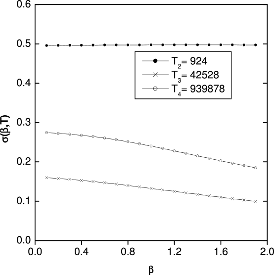
Figure 3: The behavior of the function $\sigma(\beta,T)$. During the domain forming stage $\sigma(\beta,T)=1/2$, while it is $\beta$ dependent in the domain coarsening stage. As in the example shown, $\sigma(\beta,T)$ also varies with time during the second stage.

Results shown in Figure 2 can be used to compute $\sigma(\beta,t)$. At a given time $t$, we use the five nearest points ($t$ and the closest two points on both sides) to calculate the slope of the curves $\log\delta(\beta,t)$ vs. $\log t$ using a least squares fit. As shown in Figure 3, this analysis confirms that $\sigma_{I}(\beta,t)=1/2$ during stage I.

The onset of stage II coincides with the saturation of the peak value of the field $u({\bf x},t)$ and beyond this time the relaxation of $\delta(1.0,t)$ is slower. Further, as seen from Figure 3, $\sigma(\beta,t)$ varies both with $t$ and $\beta$. The variation with $\beta$ implies that the wave numbers associated with $\delta^{\prime}(\beta,t)$ decay at rates which depend on $\beta$; i.e., lengthscales associated with multiple features of these patterns grow at different rates golAsha . The spatio-temporal dynamics shown in Figure 1 retains this feature even for very large times, when the pattern consists of a few large domains.

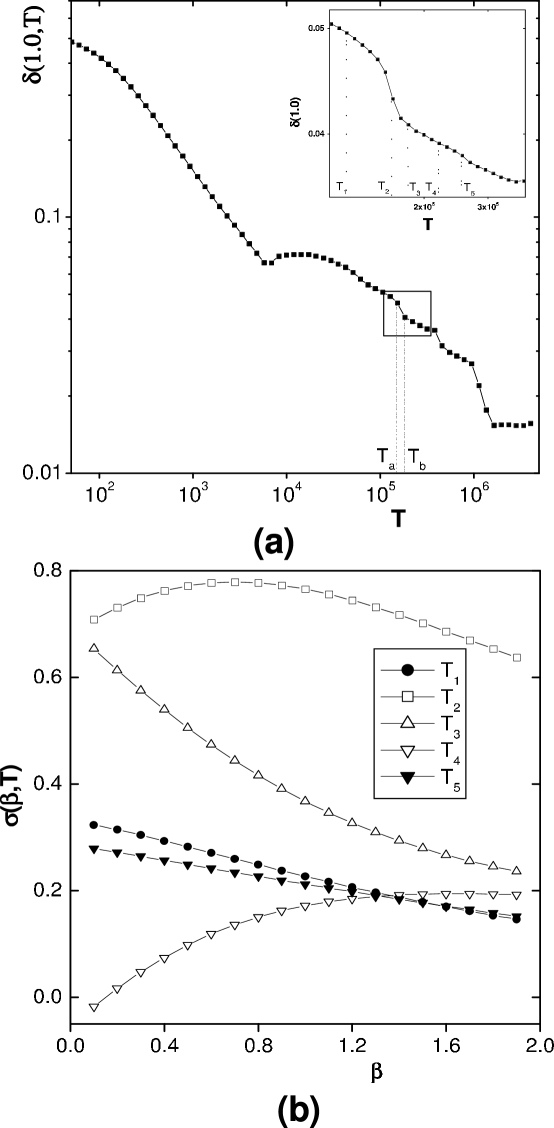
Figure 5: The behavior of $\delta(\beta,t)$ and $\sigma(\beta,t)$ during the removal of a small domain. Notice that, while $\sigma(\beta,t)$ decreases monotonically before the event and following the relaxations of the neighborhood, it exhibits more complex behavior during the event.

Typically, $\sigma(\beta,t)$ is a monotonically decreasing function of $\beta$ during stage II; thus, the mean distance between defects ($\beta\rightarrow 2$ gunAjon ) grows at a slower rate than (for example) the mean curvature or domain size. Exceptions occur during the removal of defect(s) or small domains from a pattern. These events can be identified by a sudden rapid decrease in $\delta(\beta,t)$, an example of which is seen near $T_{4}$ in Figure 2. Figure 4 shows the pattern prior to and following the absorption of a small domain into a larger one. The behaviors of $\delta(1.0,t)$ and $\sigma(\beta,t)$ during this metamorphosis is shown in Figure 5(a) and (b). It can be seen that $\sigma(\beta,t)$ which is monotonic before and after the change takes on a more complex form during the transition. This method can be used to identify domain disappearance even when it is difficult to recognize the change visually (as often happens in patterns with a large number of domains).

III Results from the Experiment

The pattern forming experiments were conducted with 0.165 mm bronze spheres contained in a vertically oscillated circular container with a diameter of 140 mm melAumb ; golAsha . The layer is four particle diameters deep, and the cell is evacuated to 4 Pa so that hydrodynamic interaction between the grains and surrounding gas is negligible. The control parameters are the frequency $f$ of the sinusoidal oscillations and the peak acceleration of the container relative to gravity, $\Gamma=(2\pi f)^{2}A^{2}/g$, where $A$ is the amplitude of the oscillation and $g$ is the gravitational acceleration. As $f$ and $\Gamma$ are changed, a variety of temporally subharmonic patterns including locally square, striped, or hexagonal patterns are observed melAumb . The textures analyzed consisted of patterns with square planforms golAsha .

The granular surface is visualized by illuminating the cell using a ring of LEDs surrounding the cell and is strobed at the drive frequency of the container. The light is incident at low angles and the scattering intensity is a nonlinear function of the height of the layer; scattering from peaks (valleys) creates bright (dark) regions.This intensity field is used to represent the structures golAsha .

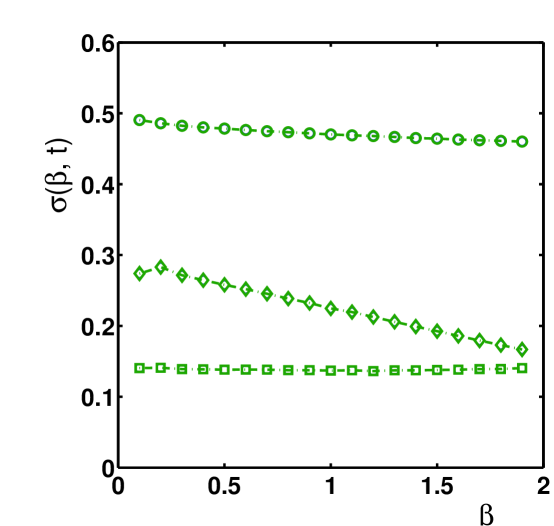
Figure 8: $\sigma(\beta,T)$ calculated for patterns shown in Figure 6. Results from stages I, II, and III are shown in circles, diamonds and squares respectively. $\sigma(\beta,t)$ for the three stages were calculated using intervals shown in Figure 6 (3-5 oscillations, 40-50 oscillations, and 85-105 oscillations following the initiation of the experiment). Now stages II and III can clearly be delineated.

Figure 6 shows four snapshots during the evolution of an experimental pattern, and Figure 7 shows the corresponding behavior of $\delta(1.0,t)$. Stages I and II, analogous to those seen in patterns of the model system, can be observed. It was confirmed that the onset of stage II corresponded to the saturation of the peak amplitude golAsha . Using the leftmost interval shown in Figure 7, the evolution during stage I was shown to be consistent with $\sigma(\beta,t)=1/2$, although there were insufficient data points for the result to be conclusive golAsha . Beyond this stage, the relaxation was much slower, and $\sigma(\beta,t)$ depends on $\beta$ golAsha , see Figure 8. However, it was observed that at much longer times (e.g., during the rightmost interval in Figure 7) the patterns reach a stage where $\sigma(\beta,t)$ is independent of $\beta$, and its value is not the universal 1/2 of the first stage, see Figure 8.

IV Spatio-temporal Dynamics under Stochastic Equations

Behavior analogous to stage III in experimental patterns is not observed in the spatio-temporal dynamics such as that shown in Figure 1, even at very large times when the pattern consists of a few domains. Clearly, one or more ingredients that are necessary for the description is missing from the model we have used. Candidates include non-variational terms, finite size effects and stochastic terms. In particular, only finite subdomains of the experimental system are analyzed (in contrast the model system has periodic boundary conditions), and stochasticity has been shown to play a role in the dynamics near the onset of patterns golAswi .

Integration of the model system shows that neither the addition of non-variational terms ($\nu\neq 0$) to the spatio-temporal dynamics nor conducting the analysis on smaller sub-domains give a transition away from stage II, even at very large times. On the other hand, we find that the addition of stochastic terms does lead to such a transition, and that the new stage has characteristics described in the last section.

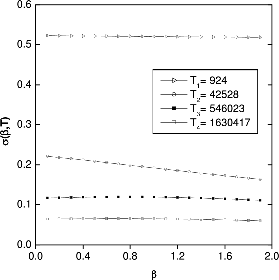
Figure 10: The behavior of $\sigma(\beta,T)$ for stochastic spatio-temporal dynamics. Observe the presence of three distinct stages, as in experimental patterns.

Figure 9 shows four snapshots during the development of such a structure under the Swift-Hohenberg equation with stochastic terms (i.e., $F\neq 0$). The behavior of $\delta(1.0,t)$ is qualitatively similar to Figure 2. The principal difference that can be gleaned from the analysis of a single moment $\delta(\beta,t)$ is an increase in the decay rate, particularly in stage II. $\sigma(\beta,t)$ exhibits features that are similar to the corresponding noise-free dynamics; it is independent of $\beta$ in stage I, but is a function of $\beta$ following saturation of the field $u({\bf x},t)$. However, at very large times, $\sigma(\beta,t)$ is once again seen to be independent of $\beta$, taking a value that depends on control parameters, see Figure 10. It is also found that the onset of stage III advances with increasing intensity of the stochastic terms. For sufficiently large values of $F$ the dynamics can move directly from stage I to III.

The implication of the $\beta$ independence of $\sigma_{III}$ is that all lengthscales associated with the pattern grow at the same rate during stage III. This assertion can be tested by studying the relaxation of the width of the structure factor and the defect density. For the analysis, we used averages for four nominally identical runs with parameters given in Figure 9. The mean decay rate of the width of the structure factor at time $T_{3}$ of Figure 10 is found to be $0.119\pm 0.014$, in agreement with $\sigma_{III}(T_{3})$. Secondly, the mean number of defects at $T_{3}$ (XX HOW WAS THIS CALCULATED?) is found to decrease like $T^{\chi}$, where $\chi=-0.201\pm 0.019$. The associated lengthscale (i.e., the mean distance between defects) grows with an index $\frac{1}{2}\chi$, once again consistent with the value of $\sigma_{III}(T_{3})$.

V Discussion and Conclusions

We set out to compare and contrast pattern dynamics in distinct systems. It is important to note that such a task can only be achieved using “configuration independent” characteristics; i.e., measures that depend on control parameters of the underlying system, and not on the (random) initial states. For complex patterns with local planforms such as stripes, squares or hexagons (e.g., Figures 1, 6 and 9), such measures include the width of the structure factor eldAvin ; croAmei , defect density houAsas , length of domain boundaries ouyAswi2 , and the disorder function gunAjon ; gunAhof .

Analysis of patterns generated in the Swift-Hohenberg equation and on a vibrated layer of brass beads show that during early times all components of the disorder function relax as $t^{-0.5}$. We showed that the index can be obtained by noting that during this stage the intensity of the field representing the pattern is sufficiently small and hence the spatio-temporal dynamics can be considered to be linear. The saturation of the field is followed, in each case, by a second stage where the relaxation is non-universal and the growth indices $\sigma(\beta,t)$ are $\beta$ dependent; the latter implies that the growth of distinct features of patterns occur at different rates. Experimental patterns exhibit a third stage at times very long compared to the vibrational period of the container golAsha , where $\sigma(\beta,t)$ is once again independent of $\beta$. It is not possible to differentiate it from stage II by analyzing the behavior of a single index; rather, it requires the use of the entire family of indices $\sigma(\beta,t)$. Unlike in stage I, the value of $\sigma(\beta,t)$ is not universal. Stage III is not present in spatio-temporal dynamics under the non-stochastic Swift-Hohenberg equation, even when non-variational terms and finite-size effects are included. Our work suggests that the ingredient required to initiate stage III is stochasticity of the underlying spatio-temporal dynamics.

It should be noted that $\delta(\beta,t)$ was constructed to quantify disorder in patterns that consist of local planforms which satisfy the Helmholtz equation gunAhof . Structures formed in other systems, such as in the X-Y model bray , in spinodal decomposition cahAhil , or in epitaxial growth vveAzan do not have such local planforms. Measures to conduct irreversible statistical analyses of such structures remain to be identified.

The authors would like to acknowledge discussions with M. Shattuck. This research is supported by grants from the National Science Foundation (DJK, GHG), the R. A.. Welch Foundation (DJK), and the Office of Naval Research (GHG).

Figure 1: Four snapshots of the spatio-temporal dynamics of a random initial state ($|u({\bf x},t)|<0.001$) under Eqn. 2 with $D=0.01$, $\epsilon=0.1$, $k_{0}=3$, and $F=0$. Times $T_{1}=124$ and $T_{2}=924$ are in stage I, and $T_{3}=42,528$ and $T_{4}=939,878$ are in stage II.

Figure 2: The behavior of $\delta(1.0,T)$ for the spatio-temporal dynamics shown in Figure 1. The presence of two distinct stages of relaxation can clearly be observed.

Figure 4: Sharp reductions in $\delta(\beta,T)$ (similar to that near $T_{4}$ in Figure 1) correspond to the disappearance of domains or defects. The images (a) before, and (b) after such an event. It is found that $\sigma(\beta,T)$ fails to be monotonically decreasing during and immediately following such events.

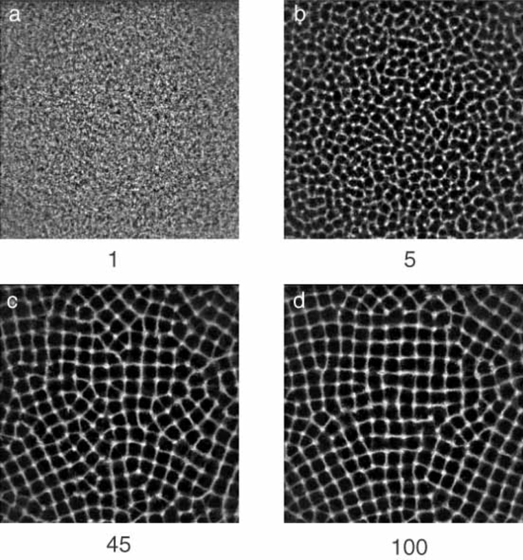
Figure 6: the time evolution of an oscillated layer of grains following a rapid change in peak acceleration of the container from $2.2g$ to $3.0g$. Below the onset of patterns (which occurs at approximately $2.5g$), the layer is featureless but noisy while above onset defect-free square patterns are stable. The numeral below each snapshot indicates the number of layer-plate collisions after the last layer takeoff before the acceleration was changed. The oscillation frequency in this experiment is $f=27$ Hz.

Figure 7: The time evolution of $\delta(1.0)$ for the sequence shown in Figure 6. The abscissa is in units of the number of container oscillations from the last layer takeoff take before $\Gamma$ was changed. The dashed lines indicate the time that snapshots in Figure 6 were taken. Two distinct stages of pattern evolution are clearly visible; the initial rapid decay is consistent with $t^{-0.5}$, while the slower decay scales on average like $t^{-0.12}$. However, it is difficult to differentiate stages II and III from the dynamics of a single moment of the disorder function.

Figure 9: Four snapshots of the stochastic spatio-temporal dynamics of a random initial state ($|u({\bf x},t)|<0.001$) under Eqn. 2 with $\epsilon=0.01$, $k_{0}=3$, and $F=0.0001$. The $T_{1}=924$ ls in stage I, $T_{2}=45,528$ in stage II, and the last two $T_{3}=546,023$ and $T_{4}=1,630,417$ are in stage III. Note that the pattern continues to evolve, albeit slowly, in stage III.

References

- (1) M. C. Cross and P. C. Hohenberg, Rev. Mod. Phys. 65(3), 851 (1993).
- (2) D. Egolf and H. Greenside, Phys. Rev. Lett., 74, 1751 (1995).
- (3) T. Petrosky, I. Prigogine, and S. Tasaki, Physica A, 173, 175 (1991).
- (4) T. Petrosky and I. Prigogine, Proc. Natl. Acad. Sci., 90, 9393 (1993).
- (5) H. H. Hasegawa and W. C. Saphir, Phys. Lett. A, 161, 471 (1992).
- (6) I. Antoniou and S. Tasaki, J. Phys. A, 26, 73 (1993).
- (7) Q. Ouyang and H. L. Swinney, Nature (London) 352, 610 (1991).
- (8) M. S. Heutmaker and J. P. Gollub, Phys. Rev. A 35, 242 (1987).
- (9) E. Bodenschatz, J. R. de Bruyn, G. Ahlers, and D. S. Cannel, Phys. Rev. Lett. 67, 3078 (1991).
- (10) R. E. Rosenweig, Ferrohydrodynamics (Cambridge University Press, Cambridge, 1985).
- (11) F. Melo, P. Umbanhower, and H. L. Swinney, Phys. Rev. Lett. 72, 172 (1993).
- (12) M. Bestehorn, Phys. Rev. E 48, 3622 (1993).
- (13) K. R. Elder, J. Viñals, and M. Grant, Phys. Rev. A 46, 7618 (1990).
- (14) H. R. Schober, E. Allroth, K. Schroeder, H. Müller-Krumbhaar, Phys. Rev. A 33, 567 (1986).
- (15) M. C. Cross and D. I. Meiron, Phys. Rev. Lett. 75, 2152 (1995).
- (16) Q. Hou, S. Sasa, and N. Goldenfeld, Physica A 239, 219 (1997).
- (17) D. Ruelle, “Statistical Mechanics, Thermodynamic Formalism,” Addison-Wesley, Reading, Massachusetts, 1978; M. J. Feigenbaum, J. Stat. Phys., 46, 919 (1987).
- (18) G. H. Gunaratne, R. E. Jones, Q. Ouyang, and H. L. Swinney, Phys. Rev. Lett. 75, 3281 (1995).
- (19) G. H. Gunaratne, A. Ratnaweera, and K. Tennekone, Phys. Rev. E 59, 5058 (1999).
- (20) D. I. Goldman, M. D. Shattuck, H. L. Swinney, and G. H. Gunaratne, Physica A, 306, 180 (2002).
- (21) D. K. Hoffman, G. H. Gunaratne, D. S. Zhang, and D. J. Kouri, Chaos 10, 240 (2000).
- (22) J. Oh and G. Ahlers, Phys. Rev. Lett., 91, 094501 (2003).
- (23) D. I. Goldman, J. B. Swift, and H. L. Swinney, “Noise, coherent fluctuations, and the onset of order in an oscillated granular fluid,” cond-mat/0308028 at arXiv.
- (24) Methods used to integrate these spatio-temporal dynamics are described in Ref. gunArat .
- (25) These integrals cannot be calculated due to the nonanalyticity of . The values for the analytic case, , are easily obtained using Parseval’s theorem.
- (26) A. C. Newell and J. A. Whitehead, J. Fluid Mech. 38, 279 (1969); L. A. Segel, J. Fluid Mech. 38, 203 (1969).
- (27) G. H. Gunaratne, Phys. Rev. Lett. 71, 1367 (1993); G. H. Gunaratne, Q. Ouyang, and H. L. Swinney, Phys. Rev. E, 50, 2802 (1994).
- (28) Q. Ouyang and H. L. Swinney, Chaos, 1, 411 (1991).
- (29) G. H. Gunaratne, D. K. Hoffman, and D. J. Kouri, Phys. Rev. E, 57, 5146 (1998).
- (30) A. J. Bray, Advances in Physics, 3, 357 (1994).
- (31) J. W. Cahn and J. E. Hilliard, J. Chem. Phys., 28, 258 (1958).
- (32) D. D. Vvedensky, A. Zangwill, C. N. Luse, and M. R. Wilby, Phys. Rev. E, 48, 852 (1993).