Perturbation Theory for the Double–Sine–Gordon Equation

Abstract

This paper presents the perturbation theory for the double–sine–Gordon equation. We received the system of differential equations that shows the soliton parameters modification under perturbation’s influence. In particular case $\lambda=0$ the results of the research transform into well-known perturbation theory for the sine–Gordon equation.

Keywords: Double–sine–Gordon equation, perturbation theory, soliton.

Pacs Numbers: 02.30.Jr, 05.45.Lj.

Introduction

The double–sine–Gordon (DSG) equation was studied in some physical problems. It describes spin waves in superfluid 3He, self-induced transparency in accounting degeneracy of atomic levels [1], electromagnetic waves propagation in semiconductor quantum supelattices [2], etc. The unperturbed DSG-equation can be written as

$${{\partial^{2}\varphi}\over{\partial t^{2}}}-{{\partial^{2}\varphi}\over{\partial x^{2}}}+\sin\varphi+\lambda\sin 2\varphi=0.$$ (1)

DSG-equation can not be solved with the inverse scattering transform. But it is known that equation (1) has the kink solution

$$\varphi=2\arctan\left(\sqrt{2\lambda+1}\sinh^{-1}\left({\sqrt{2\lambda+1}\over\sqrt{1-u^{2}}}(x-x_{0}-ut)\right)\right).$$ (2)

We shall call this solution as DSG-soliton, to differ it from the soliton of the sine-Gordon (SG) equation (particular case of the DSG-soliton, when $\lambda=0$). Interactions of solitary waves like (2) are not elastic [3, 4, 5], they are accompanied by the radiation loss. The propagation media also influences the soliton parameters (its speed $u$ and its location $x_{0}$). This influence can be described as perturbation in (1). Thus, we have

$${{\partial^{2}\varphi}\over{\partial t^{2}}}-{{\partial^{2}\varphi}\over{\partial x^{2}}}+\sin\varphi+\lambda\sin 2\varphi=\varepsilon f.$$ (3)

The solution (2) does not exactly satisfy (3). But if the perturbation is small we can take the DSG-soliton with slowly varying parameters as the solution. Then we find equations, which describe modifications of $u$ and $x_{0}$. For this purpose we construct the perturbation theory.

Perturbation theory (main algorithm)

This paper is not the first attempt to solve the perturbed DSG-equation. This problem was examined in assumption $\lambda\ll 1$ [6] using the inverse scattering transform for the perturbed sine–Gordon equation. But the paper did not show the DSG-soliton parameters modification.

There is a number of methods for the perturbation theory constructing [7]-[11]. As it was shown in [12] the perturbation theory for the SG-equation by McLaughlin and Scott describes the experimental results and the numerical solutions of the SG-equation better. Therefore, we use the algorithm represented in [13]. For these purposes we modify and adopt this algorithm for the DSG-equation.

Let’s rewrite the DSG-equation in matrix form

$$\partial_{t}\left[\begin{array}[]{c}\varphi\\ \varphi_{t}\\ \end{array}\right]+\left[\begin{array}[]{cc}0&-1\\ -\partial_{xx}+\sin(\circ)+\lambda\sin(2\ \circ)&0\\ \end{array}\right]\left[\begin{array}[]{c}\varphi\\ \varphi_{t}\\ \end{array}\right]=\varepsilon\left[\begin{array}[]{c}0\\ f(\varphi)\\ \end{array}\right].$$ (4)

We mark the column $(\varphi,\varphi_{t})$ as $W$

$$W=\left[\begin{array}[]{c}\varphi\\ \varphi_{t}\\ \end{array}\right].$$ (5)

$W$ is the function of the DSG-soliton parameters $u$ and $x_{0}$. So, $W=W(u,x_{0})$ or $W=W(p)$, where $p=(u,x_{0})$. We suppose that the solution of the equation (3) can be presented as

$$W=W_{0}+\varepsilon W_{1}.$$ (6)

Here $W_{0}$ is the exact solution of (1) with the dependent on time parameters.

If we insert this perturbed solution into (4) and linearize it, then we rewrite it in the following form

$$L(W_{1})=F(W_{0}).$$ (7)

Here $L$ is the linear operator which is given as

$$L=\left[\begin{array}[]{cc}1&0\\ 0&1\\ \end{array}\right]\partial_{t}+\left[\begin{array}[]{cc}0&-1\\ -\partial_{xx}+\cos\varphi_{0}+2\lambda\cos 2\varphi_{0}&0\\ \end{array}\right].$$ (8)

The right part of (7) represents the ’effective force’

$$F(W_{0})=f(W_{0})-{1\over\varepsilon}\sum_{i=1}^{2}{{\partial p_{i}}\over{\partial t}}{{\partial W_{0}}\over{\partial p_{i}}}.$$ (9)

The boundedness condition for $W_{1}$ is provided with the orthogonality $F$ to the discrete subspace of the kernel $N_{d}(L^{+})$, where $L^{+}$ is the adjoint operator to $L$

$$L^{+}=-\left[\begin{array}[]{cc}1&0\\ 0&1\\ \end{array}\right]\partial_{t}+\left[\begin{array}[]{cc}0&-\partial_{xx}+\cos\varphi_{0}+2\lambda\cos 2\varphi_{0}\\ -1&0\\ \end{array}\right].$$ (10)

Inserting the basis in $N_{d}(L^{+})$ and putting it into (9) we derive the equation, that satisfies the orthogonality condition

$$\sum_{j=1}^{2}\left(b_{i},{{\partial W_{0}}\over{\partial p_{j}}}\right){{dp_{j}}\over{dt}}=\varepsilon(b_{i},f),\ \ \ i=1,2,$$ (11)

where $\left(F(x),G(x)\right)=\int_{-\infty}^{\infty}F^{T}(x)G(x)dx$. And $b_{i}$ are the basis vectors of the adjoint space

$$b_{i}=\left[\begin{array}[]{cc}0&-1\\ 1&0\\ \end{array}\right]{{dW_{0}}\over{dp_{i}}}.$$ (12)

The equation (11) represents the perturbation theory for the DSG-soliton parameters.

Analysis of the DSG-soliton motion

And now let’s consider the case of the DSG-soliton propagation. We have

$${{dW_{0}}\over{dx}}=\left[\begin{array}[]{c}\varphi_{x}\\ \varphi_{tx}\\ \end{array}\right],\ \ \ {{dW_{0}}\over{du}}=\left[\begin{array}[]{c}\varphi_{u}\\ \varphi_{tu}\\ \end{array}\right].$$ (13)

Thus, we receive the basis vectors of the adjoint space as

$$b_{1}=\left[\begin{array}[]{c}-\varphi_{tx}\\ \varphi_{x}\\ \end{array}\right],\ \ \ b_{2}=\left[\begin{array}[]{c}-\varphi_{tu}\\ \varphi_{u}\\ \end{array}\right].$$ (14)

It allows us rewriting the system (11)

$$\left\{\begin{array}[]{l}\left(\left[\begin{array}[]{c}-\varphi_{tx}\\ \varphi_{x}\\ \end{array}\right],\left[\begin{array}[]{c}-\varphi_{u}\\ \varphi_{tu}\\ \end{array}\right]\right)\displaystyle\frac{du}{dt}=\varepsilon\left(\left[\begin{array}[]{c}-\varphi_{tx}\\ \varphi_{x}\\ \end{array}\right],\left[\begin{array}[]{c}0\\ f(\varphi_{0})\\ \end{array}\right]\right),\\ \\ \left(\left[\begin{array}[]{c}-\varphi_{tu}\\ \varphi_{u}\\ \end{array}\right],\left[\begin{array}[]{c}-\varphi_{x}\\ \varphi_{tx}\\ \end{array}\right]\right)\displaystyle\frac{dx_{0}}{dt}=\varepsilon\left(\left[\begin{array}[]{c}-\varphi_{tu}\\ \varphi_{u}\\ \end{array}\right],\left[\begin{array}[]{c}0\\ f(\varphi_{0})\\ \end{array}\right]\right).\\ \end{array}\right.$$ (15)

The other summands in (11) equal to zero. If we transfer these equations into integral form we receive

$$\left\{\begin{array}[]{l}\left(\displaystyle\int_{-\infty}^{\infty}(\varphi_{tu}\varphi_{x}-\varphi_{tx}\varphi_{u})dx\right)\displaystyle\frac{du}{dt}=\varepsilon\displaystyle\int_{-\infty}^{\infty}f(\varphi_{0})\varphi_{x}dx,\\ \\ \left(\displaystyle\int_{-\infty}^{\infty}(\varphi_{tx}\varphi_{u}-\varphi_{tu}\varphi_{x})dx\right)\displaystyle\frac{dx_{0}}{dt}=\varepsilon\displaystyle\int_{-\infty}^{\infty}f(\varphi_{0})\varphi_{u}dx.\\ \end{array}\right.$$ (16)

These equations transform into a system of two equations. They describe the evolution of soliton parameters, its speed and location.

$$\left\{\begin{array}[]{l}\displaystyle\frac{du}{dt}=-\varepsilon\displaystyle\frac{1-u^{2}}{2}\frac{2\lambda+1}{k(\lambda)}\int_{-\infty}^{\infty}f(\varphi_{0})\displaystyle\frac{\cosh(\theta)}{\cosh^{2}(\theta)+2\lambda}dx,\\ \\ \displaystyle\frac{dx_{0}}{dt}=u-\varepsilon\displaystyle\frac{u\sqrt{1-u^{2}}}{2}\frac{2\lambda+1}{k(\lambda)}\int_{-\infty}^{\infty}f(\varphi_{0})\displaystyle\frac{\theta\cosh(\theta)}{\cosh^{2}(\theta)+2\lambda}dx.\\ \end{array}\right.$$ (17)

Here $\theta=\sqrt{\displaystyle\frac{2\lambda+1}{1-u^{2}}}(x-x_{0}-ut)$, $k(\lambda)=\sqrt{2\lambda+1}+\displaystyle\frac{1}{\sqrt{2\lambda}}\tanh^{-1}\left(\sqrt{\displaystyle\frac{2\lambda}{2\lambda+1}}\right)$.

If we put $\lambda=0$, then $k(0)=2$ and this system reduces to a similar system for the perturbed SG-equation [13]. It’s easy to notice, that the parameters modification depends on the value of $\lambda$ and the type of perturbation function $f(\varphi_{0})$. This function can be written in different variations. But the most frequently appeared perturbation function contains three summands

$$f(\varphi)=-\gamma-\alpha\frac{\partial\varphi}{\partial t}-\mu[\sin(\varphi)+\lambda\sin(2\varphi)]\delta(x).$$ (18)

The influence of the constant energy pumping (the summand of $\gamma$), the energy losses (the summand with $\alpha$) and the presence of the inhomogeneous region (like the microshort in the Josephson junctions) are represented in this perturbation function. If we take $\mu=0$ and substitute the expression of (18) in (17), we shall get the following system of differential equations

$$\left\{\begin{array}[]{l}\displaystyle\frac{du}{dt}=\displaystyle\frac{\pi\gamma}{2k(\lambda)}\left(1-u^{2}\right)^{3/2}-\alpha u\left(1-u^{2}\right),\\ \\ \displaystyle\frac{dx_{0}}{dt}=u.\\ \end{array}\right.$$ (19)

Analyzing this system we derive the speed stability condition. To satisfy the condition the right part of the first equation must be equal to zero

$$\frac{\pi\gamma}{2k(\lambda)}\left(1-u^{2}\right)^{3/2}-\alpha u\left(1-u^{2}\right)=0.$$ (20)

So, we get the stabilized speed value

$$u_{0}=\frac{1}{\sqrt{1+\left(\displaystyle\frac{2k(\lambda)\alpha}{\pi\gamma}\right)^{2}}}.$$ (21)

This expression shows that if the energy pumping is minimal ($\gamma\rightarrow 0$) the soliton speed reduces to 0. On the contrary if the DSG-soliton takes the energy much faster than it looses ($\gamma\gg\alpha$) its speed increases up to 1. Putting $\lambda=0$ we take the expression for the stabilized speed of the SG-soliton [13]. Any DSG-soliton reaches the speed of $u_{0}$ under the action of energy pumping and energy loss without the difference of its initial speed.

In case $\mu\neq 0$ the system (17) can be written as

$$\left\{\begin{array}[]{l}\displaystyle\frac{du}{dt}=\displaystyle\frac{\pi\gamma}{2k(\lambda)}\left(1-u^{2}\right)^{3/2}-\alpha u\left(1-u^{2}\right)+\mu\left(1-u^{2}\right)g(\theta_{0})\\ \\ \displaystyle\frac{dx_{0}}{dt}=u-\mu ux_{0}\sqrt{2\lambda+1}g(\theta_{0}).\\ \end{array}\right.$$ (22)

Here $\theta_{0}=\sqrt{\displaystyle\frac{2\lambda+1}{1-u^{2}}}x_{0}$ and $g(x)=\displaystyle\frac{(2\lambda+1)^{5/2}}{2k(\lambda)}\displaystyle\frac{\cosh^{2}(x)-2\lambda}{\left(\cosh^{2}(x)+2\lambda\right)^{3}}\sinh(2x)$.

If we put the values $\gamma=0$ and $\alpha=0$, then we shall get the case of the pure interaction between the DSG-soliton and the inhomogeneity. The DSG-solitons with low speed reflects from the inhomogeneity. And high speed solitons overcomes this region. The results of interactions are shown on Figure 1.

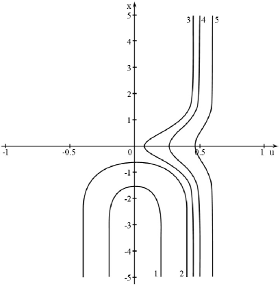
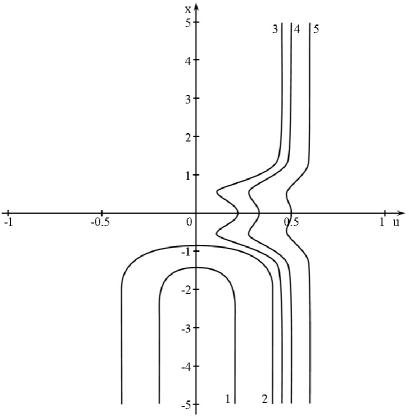
Figure 1: The DSG-soliton interaction with the inhomogeneity. The parameters are $\lambda=$ 0.2 (left), 1.2 (right); $\mu=0.5$, $\gamma=\alpha=0$. The initial soliton speed: 1) 0.2; 2) 0.4; 3) 0.45; 4) 0.5; 5) 0.6.

It is possible to find the condition of overcoming from the energy analysis. The Hamiltonian function of the unperturbed DSG-equation is defined as

$$H=\int_{-\infty}^{\infty}\left(\frac{\varphi_{t}^{2}}{2}+\frac{\varphi_{x}^{2}}{2}+(1-\cos\varphi)+\frac{\lambda}{2}(1-\cos 2\varphi)\right)dx.$$ (23)

Substituting (2) into (23) we receive the expression for the full soliton energy

$$E=\frac{4k(\lambda)}{\sqrt{1-u^{2}}}.$$ (24)

To find the ’energy of rest’ let’s put the speed value which is equal to 0. Thus, we get the kinetic energy of the DSG-soliton

$$E_{k}=4k(\lambda)\left(\frac{1}{\sqrt{1-u^{2}}}-1\right).$$ (25)

The inhomogeneous area can accumulate energy. This process can be counted as the correction to the DSG-Hamiltonian

$$H_{i}=\int_{-\infty}^{\infty}\mu\left((1-\cos\varphi)+\frac{\lambda}{2}(1-\cos 2\varphi)\right)\delta(x)dx.$$ (26)

Having substituted (2) into the previous expression we get this correction

$$H_{i}=2\mu(2\lambda+1)^{2}\left(\frac{\cosh\theta_{0}}{\cosh^{2}\theta_{0}+2\lambda}\right)^{2}.$$ (27)

The maximal energy which can be accumulated by the inhomogeneity

$$H_{max}=\left\{\begin{array}[]{ll}2\mu,&\mbox{if}\ -0.5<\lambda<0.5;\\ &\\ \displaystyle\frac{(2\lambda+1)^{2}}{4\lambda}\mu,&\mbox{if}\ \lambda>0.5.\\ \end{array}\right.$$ (28)

The value of the critical speed can be found from the condition of equality of the kinetic energy (25) and the energy accumulated in the inhomogeneity (28).

$$u_{c}=\sqrt{\frac{H_{max}^{2}+8H_{max}k(\lambda)}{[H_{max}+4k(\lambda)]^{2}}}.$$ (29)

The one more thing must be mentioned about the DSG-soliton interaction with inhomogeneity. If all media parameters ($\gamma$, $\alpha$, $\mu$) are not equal to zero the phase path is not symmetric concerning the $u$-axis. This effect is shown on Figure 2.

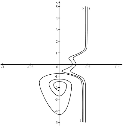
Figure 2: The DSG-soliton interaction with inhomogeneity in case $\alpha=0.04$, $\mu=0.5$, $\lambda=1.2$, $\gamma$: 1) 0.030; 2) 0.032; 3) 0.035.

This asymmetry is caused by the energy pumping presence. As soon as the soliton begins to loose its speed the equilibrium condition (20) breaks. From this moment the system has the positive balance of the energy gain. This process changes the DSG-soliton speed and, therefore, the phase path changes its shape. This effect takes place in the same problem for the SG-equation, but usually it isn’t considered. The asymmetry is small if the media parameters $\alpha$, $\gamma\ll 1$ or the soliton speed $u\rightarrow 1$.

In addition to this effect we notice the soliton damping after reflection. The damping is caused by the influence of energy inflow that pulls the solitary wave to the positive direction along the $x$-axis.

The numerical analysis shows that the view of the phase path depends on the value of the $\lambda$-parameter (see Figure 3).

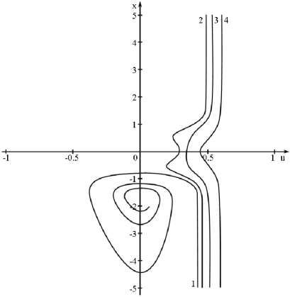
Figure 3: The influence of $\lambda$ on the DSG-soliton motion in case $\gamma=0.035$, $\alpha=0.04$, $\mu=0.5$, $\lambda$: 1) -0.2; 2) 0.5; 3) 1.2; 4) 1.9.

It is necessary to notice that the condition (28) allows to classify the DSG-solitons. The DSG-soliton (exactly, its derivative) looks like one-humped solitary wave (like the SG-soliton), when $\lambda\in(-0.5,0.5)$. If $\lambda>0.5$, the DSG-soliton is a two-humped wave. That’s why the phase path has two turning points if . And the phase path has the only one extreme point in case $\lambda<0.5$. Thus, it is possible to evaluate the $\lambda$-parameter observing the soliton behaviour. And vice versa. We can control the propagation process by changing the value of $\lambda$.

Conclusion

In the conclusion we shall briefly observe some results. First of all, this paper contains the perturbation theory that has been adopted for the DSG-equation. The derived formulas were used to consider the DSG-soliton propagation. It is shown that the DSG-soliton can be stabilized in the presence of the constant energy pumping and energy loss. We derive the condition of the stabilization. Also the DSG-soliton interaction with inhomogeneity was studied. We notice two variants of interaction: reflection and overcoming. And so we receive the condition of their separation. The variant of the propagation depends on the parameters of the media: $\alpha$, $\gamma$, $\mu$ and $\lambda$.

In case $\lambda=0$ all the results transform into the same expressions for the SG-equation [13].

Appendix A

We represent the integrals that were used in the calculations. We use $\tanh^{-1}$ to mark the inverse hyperbolic tangent. To derive these expressions well-known integrals from [dwight] were taken.

$$\int\displaystyle\frac{dx}{\cosh^{2}x+a}=\displaystyle\frac{1}{\sqrt{a(a+1)}}\tanh^{-1}\left(\sqrt{\displaystyle\frac{a}{a+1}}\tanh x\right).$$

$$\begin{array}[]{c}\displaystyle\int\displaystyle\frac{\cosh^{2}x\ dx}{(\cosh^{2}x+a)^{2}}=-\displaystyle\frac{(2a+1)e^{2x}+1}{(a+1)\left(e^{4x}+2(2a+1)e^{2x}+1\right)}-\\ -\displaystyle\frac{1}{2\sqrt{a}(a+1)^{3/2}}\tanh^{-1}\left(\displaystyle\frac{2\sqrt{a(a+1)}}{e^{2x}+2a+1}\right).\\ \end{array}$$

$$\int\displaystyle\frac{dx}{(\cosh^{2}x+a)^{2}}=\frac{1}{a}\left(\displaystyle\int\displaystyle\frac{dx}{\cosh^{2}x+a}-\displaystyle\int\displaystyle\frac{\cosh^{2}x\ dx}{(\cosh^{2}x+a)^{2}}\right).$$

The definite integrals were calculated.

$$\int_{-\infty}^{\infty}\displaystyle\frac{dx}{\cosh^{2}x+a}=\displaystyle\frac{1}{\sqrt{a(a+1)}}\tanh^{-1}\left(\sqrt{\displaystyle\frac{a}{a+1}}\right).$$

$$\int_{-\infty}^{\infty}\displaystyle\frac{\cosh^{2}x\ dx}{(\cosh^{2}x+a)^{2}}=\displaystyle\frac{1}{a+1}+\displaystyle\frac{1}{\sqrt{a}(a+1)^{3/2}}\tanh^{-1}\left(\sqrt{\displaystyle\frac{a}{a+1}}\right).$$

$$\int_{-\infty}^{\infty}\displaystyle\frac{dx}{(\cosh^{2}x+a)^{2}}=\displaystyle\frac{1}{\sqrt{a}(a+1)^{3/2}}\tanh^{-1}\left(\sqrt{\displaystyle\frac{a}{a+1}}\right)-\displaystyle\frac{1}{a(a+1)}.$$

Appendix B

There are the expressions for the function $k(\lambda)$:

a)

if $\lambda>0$, then $k(\lambda)=\sqrt{2\lambda+1}+\displaystyle\frac{1}{\sqrt{2\lambda}}\tanh^{-1}\left(\sqrt{\displaystyle\frac{2\lambda}{2\lambda+1}}\right)$;

b)

if $\lambda=0$, then $k(\lambda)=2$;

c)

if $-0.5<\lambda<0$, then $k(\lambda)=\sqrt{2\lambda+1}+\displaystyle\frac{1}{\sqrt{-2\lambda}}\arctan\left(\sqrt{\displaystyle\frac{-2\lambda}{2\lambda+1}}\right)$.

References

- [1] Salamo G.J., Gibbs H.M. and Churchill G. C., Phys. Rev. Lett., 33, 273 (1974).
- [2] Kr’uchkov S. V. and Shapovalov A. I., Sov. Optics and Spectroscopy, 2, 286 (1998).
- [3] Ablowitz M.J., Kruskal M.D. and Ladik J.F., SIAM, J. Appl. Math., 36, 428 (1979).
- [4] Bullough R.K. and Caudrey P.J., Rocky Mountain J. Math., 8, 53 (1978).
- [5] Olsen O.H. and Samuelsen M.R., Wave Motion, 4, 29-35 (1982).
- [6] Mason A.L., in: A.O. Barut, ed., Nonlinear Equations in Physics and Mathematics, Reidel Publishing Company, Dordrecht, Holland, 205-218 (1978).
- [7] Yan J., Tang Y. Zhou G. and Chen Z., Phys. Rev. E, 58, 1064-1073 (1998).
- [8] Grimshaw R., Pelinovsky E. and Bezen A., Wave Motion, 26, 253-274 (1997).
- [9] Zhang F., Phys. Rev. E, 58, 2558-2563 (1998).
- [10] Sanchez A. and Bishop A.R., SIAM Review, 40, 579-615 (1998).
- [11] Maniadis P., Tsironis G.P., Bishop A.R. and Zolotaryuk, Phys. Rev. E, 60, 7618-7621 (1999).
- [12] Salerno M., Soerensen M.P., Skovgaard O., Christiansen P.L., Wave Motion, 5, 49-58 (1983).
- [13] Solitons in Action, ed. by K. Lonngren and A. Scott, Academic Press, New York (1978).