Construction of a natural partition of incomplete horseshoes

A method is presented to construct a partition of an incomplete horseshoe in a Poincare map which is only based on unstable manifolds of outermost fixed points and eventually their limits. Thereby this partition becomes natural from the point of view of asymptotic scattering observations. The symbolic dynamics derived from this partition coincides with the one derived from the hierarchical structure of the singularities of scattering functions.

PACS number(s): 05.45.-a

1 Introduction

The most compact global description of the qualitative structure of all trajectories of a chaotic system is by giving a symbolic dynamics together with a corresponding overshadowing by basic trajectory segments. To a given symbolic dynamics there corresponds a partition of that part of the phase space which covers the chaotic invariant set. Then any trajectory is characterized by the symbol string corresponding to the sequence of partition cells visited by this trajectory. The symbolic encoding of any trajectory as a sequence of symbols allows for computing measures of chaos using the thermodynamic formalism [1]. In most cases it is easier to work with maps than with flows. Therefore we cast the system under study into some iterated map and in this map the chaotic set is represented by some version of Smale’s horseshoe [2]. Then the construction of a symbolic dynamics for the system is converted into the task to construct a partition of that part of the domain of the map which covers the chaotic set i.e. the fundamental area of the horseshoe. For simplicity in this article we only consider maps on a two dimensional domain. We think of Hamiltonian systems with two degrees of freedom which are converted into a two dimensional Poincare map.

If the horseshoe is complete then the partition is immediate and is done by a few arcs of the unstable manifolds of some of the fixed points of the map. The corresponding symbolic dynamics becomes a complete shift of symbol strings, where to each partition cell corresponds one symbol value. Problems appear if the horseshoe becomes incomplete, if pruning sets in [3] and the symbolic dynamics needs grammatical rules. Then at first sight there is no natural partition of the horseshoe area which leads to some useful symbolic dynamics. Some time ago [4]- [5] it has been proposed to use in this case as division lines the line of maximal folding of the horseshoe. It is essentially the line along which the tip of inner arcs of unstable manifolds move when we deform a complete horseshoe into the incomplete one under study by varying some parameter of the system. Later some criticism of the original method has been published [6]- [7] and in reaction to these remarks an improved version of this basic idea has been developed [8] - [9]. This improved version includes symmetry lines as parts of the division lines and is able to handle KAM islands in the horseshoe. If the task is only to construct some partition which separates trajectories, then the problem is solved by this method.

However, any method based on fold lines or, more generally, based on lines which are not given by invariant manifolds of outermost fixed points of the horseshoe leads to a completely different type of problems if we use it for the description of scattering processes [10]. Then the branching tree coming from the symbolic dynamics does not coincide with the branching tree coming from the hierarchical structure of the singularities of the scattering functions. This structure of the scattering functions is completely determined by the intersection pattern between the stable manifolds and the local segment of the unstable manifold of the outermost fixed points of the Poincare map. Level by level ( iteration step of the map by iteration step of the map ) new gaps are cut out of this local segment of the unstable manifold and these gaps correspond one to one to the intervals of continuity seen in scattering functions. Therefore the partition of the horseshoe becomes incompatible as soon as it uses any kind of division lines which are not related directly to these invariant manifolds of the outermost fixed points. Now the problem arises: Can we construct some partition of incomplete horseshoes which is exclusively based on this manifold structure and which is compatible with the branching tree derived from scattering data ?

In [10] an ad hoc solution has been given for a particular case. In the present article we show how the basic ideas for this particular solution can be converted into a general method applicable to any incomplete horseshoe. Of course, any scattering based treatment of a system can only take into account that part of the system which is accessible to the outside world and which can be seen by an asymptotic observer. Therefore our partition only takes into account the outer unstable part of the horseshoe. It ignores completely KAM islands and their interior. Near the fractal surface of KAM island and its surrounding of secondary structures it becomes approximate. We think that an approximate symbolic dynamics for a chaotic system is as valuable as an approximate analytic solution for a system which is mainly regular. This is our motivation for the detailed presentation of the method.

2 Horseshoe development stage and its appearance in scattering data

In the domain of the Poincare map $P$ the horseshoe is traced out by the invariant manifolds of the outer most fixed points. To start the horseshoe construction one defines a fundamental area $R$ which covers the whole chaotic invariant set. The choice of $R$ is not unique. We choose $R$ to be a quadrilateral whose corner points are the outer most fixed point(s) as well as other primary intersection points [11] of the invariant manifolds. Its boundary lines are segments of the invariant manifolds of the outer fixed point(s). Under iterated applications of the map the area $R$ stretches and folds resulting in a horseshoe.

The image $P(R)$ does not cover $R$ completely. It leaves some holes. Let us assume that the complement $R\setminus P(R)$ has $n-1$ connected components. Then we deal with an n-ary horseshoe having n arms. We call the various components of this complement the first level unstable gaps $g_{1,j}$ where $j$ runs from $1$ to $n-1$. The unstable gaps $g_{k,j}$ of level $k$ are the images of the first level gaps under the $(k-1)$ fold application of $P$. Stable gaps can be defined in analogy by using the inverse map. We mainly deal with the unstable gaps, therefore, if we only say gaps we mean the unstable ones. Higher level gaps can penetrate $R$ several times completely and/or several times incompletely.

The boundaries of unstable/stable gaps are given by segments of the unstable/stable manifolds of the outer fixed point(s). The gaps are areas that are not needed to cover the chaotic invariant set. A point that lies in a stable/unstable gap of level $n$ is mapped out of $R$ after $n$ applications of the map/inverse map. As we later show, we build the cells for partitioning the phase space around these unstable gaps.

The development stage of the horseshoe can be described by parameters, $\alpha_{j}$, that measure how much the gaps $g_{1,j}$ penetrate through $R$ compared to the complete case [12]. For a complete horseshoe, $g_{1,j}$ penetrate completely through $R$ and $\alpha_{j}=1$ for all $j$. The significance of these parameters is that they describe the qualitative global aspects of the outer part of the horseshoe which is accessible to scattering trajectories. They ignore the details and in particular they can not describe the secondary structures close to the surface of KAM island nor the interior of KAM islands. However, it determines quite well the outer hyperbolic part of the chaotic invariant set whose effects are contained in the scattering data. To describe the development stage of a horseshoe one needs, in general, a parameter $\alpha_{j}$ for every gap of level $1$. If the tip of $g_{1,j}$ ends inside of a stable gap ( and for arbitrary physical parameters of the system this happens with probability one ), i.e. if the map avoids primary homoclinic tangencies and if as a consequence starting from a certain level ( call it $l+1$ ) all tips of gaps end outside of $R$, then each $\alpha_{j}$ can be expressed as $k_{j}/n^{l}$ [12], where $n$ is the number of arms of the horseshoe defined above ( i.e. if we have a n-ary horseshoe ), and $k_{j}$, $l$ are integers ($k_{j}$ does not contain any factor $n$). If the system has symmetries, a smaller number of development parameters may be sufficient. For more explanation of this description of the development stage see [13].

Here we give a very brief description how we get the number $k_{j}$. For simplicity we do it for the binary case where only a single gap of level $1$ exists and where we do not need the index $j$. Let us assume that the first level unstable gap ends in some segment of the l-th level stable gap. Then this segment of the gap corresponds to some segment of the l-th level stable gap of the corresponding complete horseshoe. Then we take in the complete horseshoe all gaps up to level $l$ and count all their penetrating segments ( in the complete case there are no partial penetrations ) consecutively starting from the side of the outer fixed point. The number $k$ is the number, in the complete case, of that segment in which the unstable first level gap ends, in the incomplete case under consideration ( for more details see [13]). Note that not all numbers of the form $k/n^{l}$ correspond to existing development stages of horseshoes. In [12] it has been explained why by discussing, as an illustrative example, the nonexistence of the binary $3/8$ case.

Our method for partitioning the phase space requires the knowledge of these development parameter(s). If only asymptotic data are available, then, $\alpha_{j}$ can be obtained from the symbolic encoding of the hierarchical structure of the fractal set of singularities of the scattering function [13]-[14]. Sometimes symmetry considerations must be included, as well, to decide the basic type of the horseshoe, e.g. whether it is a binary or a ternary one.

3 Algorithm for partitioning the phase space

To avoid clumsy notation we present our method for the case of only one gap of level $1$. If the map has several ones, then for each one of them the same procedure has to be performed. In the examples we will also show ternary horseshoes with 2 gaps of level $1$. First we make the following definitions for the notation: From now on we call such segments of gaps of level $p$ which cut $R$ completely the $A_{p}$ part and ( if it exists ) the remaining part which only penetrates partially into $R$ the $B_{p}$ part ( note that $B_{p}$ is always the image of a part of $B_{p-1}$. Then there exists an integer $m$ such that for levels $1\leq p\leq m$ the whole gap $g_{p}$ only consists of one $B_{p}$ part and the level $m+1$ is the first level for which the gap contains an $A$ part and cuts $R$ completely.

At every level $p$ we define the unresolved region $U_{p}$ as that part of the fundamental area $R$ which is not yet assigned to any partition cell. In general, $U_{p}$, might consist of various components.

Before we give rules in the form of an algorithm, for partitioning the phase space, let us emphasize two principles which we must follow strictly in order to obtain a partition which coincides with the one seen by the asymptotic observer:
Principle 1 : If an arc of the unstable manifold ( i.e. boundary of a gap ) leaves $R$ and reenters $R$ then the two cells which this arc connects must be different, i.e. must belong to different symbol values, always if the preimage of the segment which leaves $R$ has completely been inside of $R$. The arc of the unstable manifold under consideration may connect the boundary of two different cells.
Principle 2 : There must be a division line between two areas inside of $R$ where the arcs of unstable gaps have qualitatively different behaviour. Thereby we mean: $R$ has two stable sides and there are segments of unstable gaps in $R$ which connect one of these stable sides with the other one. There are also segments of unstable gaps which start on one of these sides and return to the same side. Such arcs wind around some incomplete unstable cut ( $B$ part of a gap ) of lower level. The boundary between areas of these two types of behaviour must become a division line. In addition if some arcs wind around a $B_{p}$ gap and other arcs wind around a different $B_{q}$ gap then these two areas also must be separated by a division line.
In total we obtain three types of division lines. First, images of $B$ gaps ( division lines of class $1$ ). Second, boundaries of areas where arcs wind around a particular $B$ gap. The first class of division lines is defined on finite level of the hierarchy, the second case is in many cases defined by an iterative procedure in the limit of level to infinity only ( such division lines are of class $2$ ). Sometimes ( it allways happens in hyperbolic incomplete cases, but not only in them ) this division is done at a finite level ( division lines of class $3$ ). This happens if arcs of gaps make turns such that the outer boundary leaves $R$ whereas the inner boundary turns inside of $R$. If division lines of class $3$ do not occur, then the partition leads to grammatical rules of length $1$, if division lines of class $3$ exist, then the grammar may be of length larger than $1$. To get a grammar of length $1$ in such cases may require the introduction of additional division lines. They are $A$ parts of preimages of division lines of class $3$ and thereby are gaps in whose interior some tip of a stable gap ends. See the examples in the next section. Division lines of class $1$ can appear up to level $l+1$, division lines of class $3$ can appear up to level $2l$.
The algorithm can be cast into the following steps:
1. Start with the fundamental rectangle $R$. It has $2$ unstable sides, at least one of them is a local segment of an unstable manifold of an outer fixed point. The $2$ unstable sides of $R$ will later become the outer boundaries of $2$ partition cells. Already now we can assign to these boundaries the symbol values which will be assigned later to the adjacent cells. For boundaries which are local segments of unstable manifolds we use as symbol values the names of the corresponding outer fixed points, such that the corresponding cells represent these fixed points in the sense of overshadowing.
2. Define the integer $m$ as the one fulfilling the relation

$$\frac{1}{n^{m}}\leq\alpha<\frac{1}{n^{m-1}}$$ (1)

for $\alpha<1$. In the particular case of $\alpha=1$ we set $m=0$. It coincides with the $m$ mentioned above. Extend the unstable manifold level by level, i.e. construct the gaps $g_{p}$ for $p$ from $1$ up to $m$. None of these gaps will penetrate $R$ completely, i.e. none will cut $R$ into several components. Each $B$ part of a gap $g_{p}$ will become the center of a partition cell ( thereby principle 2 will be fulfilled ). We already assign the corresponding symbol value to these gaps during the construction of the levels from $1$ to $m$. Accordingly at level $m$ we have already $m+2$ different symbol values in total ( including the two symbols for the unstable sides of $R$ ).
3. The unstable gap $g_{m+1}$ is the first gap that cuts through $R$ completely and separates $R$ into at least two disconnected parts. All $A_{m+1}$ cuts must become the division lines between different cells. At least one of the parts into which $R$ is cut is a topological rectangle. At the moment we take it as one complete cell. Eventually it may be cut into several ones at higher levels. At the inner side of the cuts we assign a new symbol value which belongs to a partition cell which will be constructed on this side on higher levels. This step is a special case of the more general step 5.C explained below.
4. If $k\neq 1$ then $g_{m+1}$ contains a $B_{m+1}$ part in addition. As in step 2 this $B$ part becomes the center of a new partition cell and we have to give it a new symbol value.
5. Starting from level $m+1$ each gap cuts through $R$ completely, in general several times. And up to level $l$ it contains in addition one $B_{p}$ part close to its tip. These $B_{p}$ parts we treat as before: We assign a new symbol value to the new unstable boundary around $B_{p}$. It will become the outer unstable boundary of a partition cell. The inner boundary of the corresponding cell will be constructed at higher levels. For the various $A_{p}$ cuts we must distinguish several possibilities:
A. Such cutting segments are images of $A_{p-1}$ and run in the interior of already existing cells. Then they do not have any function for the partition at this moment. However they may be turned into division lines later, if point 7 applies to them.
B. Such cutting segments are images of $A_{p-1}$ and run through $U_{p-1}$. They cut $U_{p-1}$ into two components and one of them ( we call it the outer component ) is a quadrilateral. Then, the same symbol value holds on both sides of the cutting segment. The cell that already exists on the outer side of this cutting segment is extended towards the inner side and its inner boundary will be improved on higher levels. However, it must become a division line if it falls into the class $3$ mentioned in the discussion of principle 2. If all parts of $U_{p}$ should be topological rectangles then they become partition cells and the process stops. This happens for hyperbolic cases and for hyperbolic incomplete horseshoes this final step and its corresponding decomposition of $U$ into quadrilaterals necessarily includes division lines of class $3$.
C. Such cutting segments $A_{p}$ are the image of the $B_{p-1}$ gap. Then this $A_{p}$ segment becomes the division line between two different cells in any case. Now we must distinguish three subpossibilities:
–a) If the cutting segment cuts off from $U_{p-1}$ areas that are topological rectangles, then these rectangles are complete cells and are labelled by the symbol value which already existed on the opposite unstable side of these rectangles. We introduce a new symbol value only on the side of the cutting segment which is not a topological rectangle and start constructing a new cell whose outer boundary is the cutting segment under consideration.
–b) If the cutting segment does not cut off from $U_{p-1}$ a topological rectangle ( i.e. if on both sides polygons remain with more than four corners ) then, assign a new symbol on each side of the cutting segment under consideration. The inner boundaries of the corresponding cells will be constructed at higher levels.
–c) Also if an image of a $B$ part cuts an already existing cell into several pieces, then these pieces must become independent cells and must have different symbol values.
6. At levels $p>l+1$, the cutting segments of the $p$ level gap are always images of $A_{p-1}$ gaps. Thus, we proceed to higher levels by iteratively applying step 5.B to improve the cell boundaries iteratively.
7. If division lines of class $3$ exist and if we are interested in grammatical rules of length 1 then finally we convert gaps of type $A$ into division lines, if they fulfil the following properties: They contain tips of stable gaps. This is equivalent to being a preimage of a division line of class 3 such that the part of the division line of class $3$ which leaves $R$ has a preimage completely inside of $R$. There can only be a finite number of such additional division lines. Note that points 3 and 4 are special cases of point 5. We took them as separate points to start with simpler special cases. If we only want a minimal set of instructions for the division then we can drop points 3 and 4.

Note that step 5 is basically the realization of our guiding principle 2 and therefore it assures that scattering trajectories belonging to different intervals of continuity of the scattering functions are encoded by different symbol sequences. Case 5.B. accounts for trajectories that have been separated at a previous level while step 5.C. accounts for those that will be separated at the current level.

The grammatical rules of length one corresponding to this division of $R$ into cells are obtained by observing how any cell is covered by the images of the other cells.

4 Examples

The procedure will become clearer by doing a few examples in detail. In the following plots thick solid lines are final division lines of cells defined on a finite level. Thick broken lines are division lines in the limit of level to infinity but without taking into account nonhyperbolic effects. Dot dashed thick lines are division lines according to step 7 and division lines of class $3$.

4.1 Binary case $\alpha=1/2$

We illustrate our algorithm first for a binary horseshoe with $\alpha=1/2$. In this case, $m=1$, $k=1$ and $l=1$. For a binary horseshoe, the map has two fixed points, one of them being the outer fixed point. As a Poincare map we use the model map also used in [12]:

$$x(n+1)=x(n)+p(n),$$

$$p(n+1)=p(n)+Af(x(n+1))$$ (2)

Here $x$ is the position coordinate, $p$ is the momentum coordinate, $n$ is the discrete time, and $A$ is a free parameter. We take the force function to be:

$$f(x)=x(x-1)e^{-x}.$$ (3)

$A$ is a parameter which can be used to adjust the development stage of the horseshoe. First we use $A=3.4$ which is close to the lower end of the interval of $A$ values where a development parameter $\alpha=1/2$ is realized. As shown in [12] for this value of $A$ nonhyperbolic effects only start at very high levels of the hierarchy. Later we change $A$ to get a case of $\alpha=1/2$ where nonhyperbolic effects set in at rather low levels. In this later case we briefly discuss what kind of errors our method makes, if nonhyperbolic effects occur.

In Figs.(1a) and (1b) we draw $x$ and $p$ for half integer multiples of the time step $n$. We choose this Poincare surface of section for simplicity since with this choice of surface the $p\rightarrow-p$ transformation interchanges the stable and unstable manifolds. In Fig.(1a), we draw the stable manifold $W^{s}$ up to level $0$ and the unstable one up to level $2$. The topological rectangle $OGHI$ is the area $R$, with $O$ being the outer fixed point. The gap of level $1$, $g_{1}$, does not cut through $R$ completely. The gap of level $2$, $g_{2}$, cuts through $R$ completely once. Thus, $g_{2}$, cuts $R$ in two disconnected parts. One part is adjacent to the outer fixed point, $O$, and is topologically a rectangle. This part is already a complete partition cell and we assign to it the symbol $O$, it is the cross hatched area in Fig.(1a). The remaining part of area $R$ is $U_{2}$. $U_{2}$ has three separate unstable boundary parts. We assign to each one of them a symbol, %, & and $+$, respectively, which at higher levels becomes the symbol of the adjacent partition cells. The inner boundaries of these partition cells are not defined at level $2$. Thereby the first 5 steps of the algorithm are already done. Note that because the $g_{2}$ gap ends outside of $R$ there will never be any B parts of gaps starting from level $2$. Because $l=m$ in this particular case ( the reason is that $k=1$ ) step 5 is trivial and the rest is an iterative improvement of the inner boundaries of the cells %, & and $+$. From the application of the map we read off the following grammatical rules:
1 : $+\rightarrow O$, %, 2 :$O\rightarrow O$, % , 3 : % $\rightarrow$& , 4: & $\rightarrow+,O$.

In Fig.(1b) we draw the boundaries reached at level 6. The binary case $\alpha=1/2$ has a large KAM island around the inner fixed point at $(x=0,p=0)$. The figure demonstrates how the part of $U_{2}$ outside of this KAM island is divided into $3$ cells. In Fig.(1b) we see how iterative division lines separate segments of different behaviour. Cell % corresponds to segments which connect the lower boundary (IH) of $R$ with the upper boundary (OG) and end to the left of $B_{1}$. Cell $+$ corresponds to segments which connect the lower boundary of $R$ with the upper one and end to the right of $B_{1}$. Cell & corresponds to arcs which wind around $B_{1}$ and which start and end at the upper boundary of $R$. The behaviour in cell $O$ is qualitatively the same as in cell $+$ but must be divided because of principle $1$.

Next let us put the parameter $A$ of the interaction in Eq.2 to the value $4$, which still is the binary $\alpha=1/2$ case, but it is close to the upper limit of the A interval which belongs to $\alpha=1/2$ and therefore nonhyperbolic effects become important at rather low levels ( see section 4 in [12] ). Fig.(2a) shows that during the change of the parameter from $A=3.4$ to $A=4$ a homoclinic bifurcation has appeared. One intersection point of the case $A=3.4$ has split into the 3 intersection points indicated by the little circles in Fig.(2a). Since this homoclinic bifurcation shows up in an intersection between two tendrils of level $4$ in the interior of $R$ it results in secondary intersections of the unstable manifold at level $8$ with the local segment of the stable manifold ( if any homoclinic intersection point suffers some bifurcation, then all its images and preimages show the same type of bifurcation). This is demonstrated in Fig.(2b), where the unstable manifold at level $8$ intersects the local segment of the stable manifold at three points (indicated by squares) giving rise to a secondary tendril. It acts like a $B$ part of a primary gap and creates a new segment of unstable boundary of the cell. To take it into account properly in the symbolic dynamics and in the partition it would be necessary to introduce a new cell around this secondary tendril. However, we do not take into account these effects, we ignore them and thereby make an error, here our construction is approximate. For the creation of secondary tendrils see also figures 6 and 7 in [12].

In higher levels of the hierarchy such homoclinic bifurcations become more frequent and in the limit of level to infinity they take over in all nonhyperbolic cases. Note that they first appear in the vicinity of the large KAM island. Considering that the divisions between the cells &, %, + end in the surface of the KAM island and dive into its fractal surroundings makes it evident that the correct partition lines must approach fractal curves and start to develop wild oscillations if we go to high levels of the hierarchy beyond the level where nonhyperbolicities set in. The oscillations create all the secondary tendrils. The beginning of such wild oscillations in division lines has been shown in Fig.8 of Ref. [10] for the ternary symmetric case $\alpha_{1}=\alpha_{2}=1/3$. Our approximation replaces the complicated curve by a smooth curve making shortcuts through all fine oscillations. In all the other nonhyperbolic cases similar effects occur and in the examples that follow we do not mention them explicitely.

From this binary $\alpha=1/2$ example it should be clear how all binary $\alpha=2^{-j}$ cases are treated. For all these cases, the plot showing how we partition the phase space at level $l+1=m+1$ looks similar to Fig.(1a) with the only difference that $U_{l+1}$ contains $l$ partial penetrations of the gaps $g_{1}$ up to $g_{l}$. Accordingly $U_{l+1}$ contains $l+2$ unstable boundary components in total and we need $l+3$ partition cells in total for the horseshoe. This observation will become important later in section 5.

4.2 Binary complete case $\alpha=1$

Of course for this case the gap $g_{1}$ is the ideal division line of $R$ into two cells which are topological rectangles and it gives the standard symbolic dynamics in 2 symbol values. On the other hand we could also take the complete case as the special $m=0$ case of the sequence of cases mentioned at the end of the previous subsection. Then $m=0$ and we construct a symbolic dynamics in 3 symbol values, see Fig.(3). On level 1 the gap $g_{1}$ is the first one which divides $R$ and according to rule 3 we give two different symbol values on both sides. Formally we can consider this division line the image of $B_{0}$. We see that the side which contains the outer fixed point is a topological rectangle and assign to it the symbol O. But we do not recognize that the other half is also a rectangle and assign the symbol % on this side of $g_{1}$. As third symbol we assign & to the opposite side of $R$. Then iteratively the cells % and & are enlarged to the inside and in the limit of level to infinity their inner boundaries converge from both sides to the local branches of the unstable manifold of the inner fixed point. The grammatical rules are:
1 : $O\rightarrow O,$& , 2 : $\%\rightarrow O,$ &, 3 : $\&\rightarrow O,\%$.

The topological entropy of this symbolic dynamics is $ln(2)$ and it is a complete binary symbolic dynamics in disguise. All partition lines consist of vertical lines only which run from one stable boundary of $R$ to its opposite stable boundary. Of course we could construct an equivalent partition by using the corresponding horizontal strips and division lines. This shows that in this case global continuous stable and unstable directions exist and this indicates that this case is a uniform hyperbolic one.

4.3 Binary $\alpha=7/8$ case

We now illustrate our algorithm for the binary $\alpha=7/8$ case using a schematic plot. This is a nice example where division lines of type $3$ exist. In this case, $m=1$, $k=7$ and $l=3$. In Fig.(4), we draw the stable manifold $W^{s}$ up to level $0$ and the unstable one up to level $6$. The topological rectangle OGHI is the area $R$, with $O$ being the outer fixed point. The gap of level $1$, $g_{1}$ does not cut through $R$ completely. The gap of level $2$, $g_{2}$, cuts through $R$ completely once ($A_{2}$ part) and also cuts partially through $R$ ($B_{2}$ part). $A_{2}$ cuts $R$ in two disconnected parts. One part is adjacent to the outer fixed point, $O$, and is topologically a rectangle. This part is already a complete partition cell and we assign to it the symbol $O$, it is the cross hatched area in Fig.(4). At level $2$, the remaining area has three separate unstable parts. We assign to each one of them a symbol, $+$, % and $*$, respectively, which at higher levels becomes the symbol of the adjacent partition cells. The inner boundaries of these cells are not defined at level $2$. At level $3$, the gap $g_{3}$, cuts $R$ completely three times, parts $A_{3,1}$, $A_{3,2}$ and $A_{3,3}$, respectively, and also cuts partially through $R$, $B_{3}$ part. $A_{3,1}$ is the image of $A_{2}$ and runs through an already existing cell, $O$, it is therefore irrelevant. $A_{3,2}$ is the image of $A_{2}$ and cuts $R$ in two components. One of them is a quadrilateral and it is already labeled by the symbol $+$. Before though we assign a symbol value on the other side of $A_{3,2}$ we note that there are division lines of type $3$ in this case. That is, at level $4$ the gap $g_{4}$ cuts through $R$ completely $7$ times, parts $A_{4,1}$ up to $A_{4,7}$. Note that the inner boundary of $A_{4,3}$ and $A_{4,4}$ does not cut through $R$ while the outer boundary does. Thus, these lines are division lines of type $3$. In addition, according to step $7$ of our algorithm the preimage of parts $A_{4,3}$ and $A_{4,4}$, part $A_{3,2}$, is also a division line. So, to the outer side of $A_{3,2}$ we introduce a new symbol value, $4$. Next, $A_{3,3}$ is the image of $B_{2}$ so it is a division line and we introduce two different symbol values on either side, # and $1$, respectively. Next, $B_{3}$ is a new unstable boundary and we thus introduce a new symbol value, $2$. At level $4$, $A_{4,1}$ and $A_{4,2}$ run through already existing cells and are thus irrelevant. $A_{4,3}$ and $A_{4,4}$ are division lines of type $3$, as we have already noted, and different symbol values must be introduced on either side of them. $A_{4,3}$ cuts on its left side a quadrilateral, thus this side is now a complete cell already labeled by the symbol $1$. On the other side the symbol % already exists. On the left side of $A_{4,4}$ the partition cell % already exists and so we just introduce a new symbol value, $6$, on the other side. $A_{4,5}$ and $A_{4,6}$ are images of $A_{3,3}$. $A_{4,5}$ cuts on one side a quadrilateral and so the same symbol holds on both sides, $*$. $A_{4,6}$ also cuts a quadrilateral and so the same symbol value # holds on both sides. $A_{4,7}$ is the image of $B_{3}$ and cuts a quadrilateral on one side which is already labeled by $4$. We introduce a new symbol value on the other side of $A_{4,7}$, $5$. At level $l+1=4$ we are through assigning symbol values. But since we have divisions lines of type $3$ the cells centered around $B_{2}$ and $B_{3}$ take their final form only by considering levels up to $2l=6$. In Fig.(4), for simplicity, we only indicate those parts of gaps $g_{5}$ and $g_{6}$ that wind around $B_{2}$ and $B_{3}$. These parts are also division lines of type $3$ and they finalize the cells centered around $B_{2}$ and $B_{3}$. The grammatical rules are:
1: % $\rightarrow$ *,&,O, 2: * $\rightarrow O$,4, 3: & $\rightarrow$ #,2,1, 4: O $\rightarrow$ O,+, 5: 4 $\rightarrow$ 1, 6, 6: # $\rightarrow$ *, #, 7: 2 $\rightarrow$ 5,4, 8: 1 $\rightarrow$ #, *, 9: + $\rightarrow$ %, 10: 5 $\rightarrow$ 1, 6, 11: 6 $\rightarrow$ 5,O.

4.4 Ternary asymmetric case $\alpha_{1}=1/3$, $\alpha_{2}=1$

In Figs.(5a) and (5b) we draw the invariant manifolds of a system that describes the classical scattering of an electron from a one-dimensional inverted Gaussian potential in the presence of a strong laser field. This potential has offered considerable insight into the laser atom interactions [15]. The Hamiltonian in the Kramers-Henneberger reference frame (the frame which oscillates with a free electron in the time-periodic field) [16] is:

$$H=\frac{p^{2}}{2}-V_{0}e^{-((x+\beta_{0}\sin(\phi))/\delta)^{2}}+\omega I.$$ (4)

Note, that in Eqs.(4) we have transformed to a two-dimensional time-independent system, where the total energy is conserved. $I$ and $\phi$ are respectively the action-angle variables of the driving field and $\phi=\omega t$. $\beta(t)=\beta_{0}\sin(\omega t)=-qE_{0}/\omega^{2}$ is the classical displacement of a free electron from its center of oscillation in the time-periodic electric field $E(t)=E_{0}\sin(\omega t)$, where $T=2\pi/\omega$ is the period of the field. The parameters chosen here are $V_{0}=0.27035$, $\delta=2$, $\omega=0.65$ and $\beta_{0}=0.9$, all given in atomic units (a.u.). The $\alpha^{\prime}s$ for these parameter values are $(1/3,1)$. The outer most fixed points are located at $x\rightarrow\pm\infty$. For the left outer fixed point, $A$, we have, $\alpha=1$ and $l=0$, $m=0$. For the right outer fixed point, $C$, we have, $\alpha=1/3$ and $l=1$, $m=1$. For this driven system, the P-map is a stroboscopic plot. That is, we plot $x$ and $p$ every complete period of the field solving Hamilton’s equations of motion. We choose our Poincare surface of section to be $\phi=\pi/2$ because of symmetry reasons [17]. In Fig.(5a) we draw the stable manifolds $W^{s}$ up to level $0$ for both outer fixed points, the unstable $W^{u}$ of the fixed point $A$ up to level $1$, and the unstable $W^{u}$ of the fixed point $C$ up to level $2$. The 4-sided area $AECD$ is the area $R$. At this level, the cells adjacent to the fixed points are already complete ones and we label them $A$ and $C$ respectively. The remaining part of $R$ is the unresolved region and has three separate unstable boundary parts. We assign to each one of them a symbol, $+$, & and % respectively, which at higher levels becomes the symbol of the adjacent partition cells. The inner boundaries are not yet defined. In Fig.(5b) we draw the unstable manifolds up to level $4$ for both fixed points to demonstrate how the inner boundaries of the cells $+$, & and % are defined at higher levels through an iterative process. In Fig.(5b), we see how iterative division lines separate segments of different behaviour. Cell $+$ corresponds to segments which connect the lower boundary (AD) of $R$ with the upper boundary (EC) of $R$ and end to the left of $B_{1}$. Cell & corresponds to segments which connect the lower boundary of $R$ with the upper boundary of $R$ and end to the right of $B_{1}$. Cell % corresponds to arcs which wind around $B_{1}$ and which start and end at the lower boundary of $R$. The behaviour in cell $C$ is qualitatively the same as in cell & but must be divided because of principle $1$. The same is true for cells $A$ and $+$. At level $4$ one strip to the partition cell $+$, two strips to the cell &, and three strips to the cell % have been added. The inner boundaries of these cells will be improved iteratively at still higher levels. From Figs.(5a) and (5b), we find the grammatical rules to be 1 : $A\rightarrow A$, &, $C$ 2 : & $\rightarrow C$, % 3 : $C\rightarrow C$, % 4 : % $\rightarrow+,A$ 5 : $+\rightarrow A$, &, $C$.

In Fig.(5b) we indicate the KAM island around the inner elliptic fixed point $B$ by an invariant KAM torus quite close to the surface of the island. In the figure it is the dotted line. The fixed point $B$ itself at $x=-0.29$ and $p=0$, is marked by a square. The KAM islands and their fractal surrounding of secondary structures are the parts of the horseshoe which are not treated by our scattering oriented partition. The existence of KAM islands leads to non-hyperbolic effects such as secondary tendrils and related homoclinic tangencies, i.e. non transversal intersections, between stable and unstable manifolds [12]. For the parameters we currently consider the tangencies may show up at level $8$ and higher. Our method does not account for these additional intersections. This means that our partition can not encode the path of those trajectories that “dive” into the secondary structures around the fractal surface of stability islands and stay there for a very long time. However, it successfully accounts for short and intermediate time scales which are the ones most relevant to scattering.

5 Connection to rotation numbers of the central KAM island and to the selfpulsing effect

In [18] it is shown how the selfpulsing effect of chaotic scattering systems with horseshoes of small development parameters ( where a large scale KAM island around a central elliptic fixed point exists ) can be used for the inverse scattering problem. The method is based on a simple relation between the development parameter and the delay between adjacent pulses. This delay is just the number of steps of the map needed for a general trajectory in the vicinity of the large KAM island to encircle this island. In this section we explain how such a connection also drops out of our construction of a partition.

For simplicity let us first consider the binary case and start with the development parameter $\alpha=1/2$ for which we see the figures in section 4.1. As Fig.(1b) indicates the large KAM island ( containing the inner fixed point which is elliptic for $\alpha=1/2$ ) is surrounded by 3 different partition cells. Points in cell + and close to the boundary of the KAM island are mapped into cell % and again close to the boundary of the KAM island. Such points in turn are mapped into cell & and again close to the boundary of the KAM island. The images of such points lie in cell + and are again close to the boundary of the KAM island. In total, points close to the KAM island need 3 steps of the map to circle once around the KAM island.

Next imagine the binary case $\alpha=2^{-l}$. According to the remarks at the end of subsection 4.1 the region $U$ is surrounded by $l$ incomplete gaps $g_{j}=B_{l}$, $j=1,...,l$ all being the centers of corresponding partition cells. In addition there is a cell adjacent to the left hand unstable boundary of $R$ and one cell adjacent from the left hand side to the gap $g_{l+1}=A_{l+1}$. All such cells touch the large KAM island ( in contrast the cell O adjacent to the outer fixed point is the only cell not neighbouring this KAM island ), i.e. there are $l+2$ neighbouring cells of the central KAM island. Since $B_{p}$ is mapped into $B_{p+1}$ under the Poincare map, it should be clear that points close to the KAM island are mapped from any one of these cells into the neighbouring cell in the clockwise orientation. Therefore it takes $l+2$ steps of the map for such a trajectory to circle once around the KAM island.

For all these cases the connection between the number $N_{s}$ of steps it takes to encircle the KAM island and the development parameter $\alpha$ is

$$N_{s}=-\log_{2}(\alpha)+2$$ (5)

Finally, in the spirit of a smooth interpolation we use this equation as estimate for the rotation number of the surrounding of the central KAM island for all small values of $\alpha$. Note that such a formula does not make any sense for large values of $\alpha$ where no large central KAM island exists. However, we could apply an analogous consideration to estimate the rotation number of any other KAM island appearing for any value of $\alpha$.

In [18] we have given an estimate of this rotation number which resulted in an equation similar to Eq.5 with the only small difference that the constant was $3/2$ instead of $2$. Why this small discrepancy ? The explanation is rather simple: In [18] we were interested in trajectories in the secondary structures directly above the surface of the KAM island. In the present article we are concerned with trajectories in the globally unstable ( approximately hyperbolic ) part of the system which ends further outside of the surface of the KAM island. In general the rotation number in the KAM island and its secondary surrounding is somewhat smaller than in the region further out, therefore the small difference in the two estimates.

Let us give a very brief description of the selfpulsing effect itself and some relation to our partition. Imagine we put some blob of initial conditions into a single partition cell and close to the central KAM island but outside of it. When does a part of the trajectories leave $R$? Only the images of the cells around $B_{l}$ and $A_{l+1}$ have parts outside of $R$. The other $l$ cells around the island do not have this property. Therefore only after each complete revolution around the island, i.e. after $N_{s}$ steps of the map a pulse leaves the inner region and goes out to the asymptotic region where in a scattering experiment the time delay $N_{s}$ between adjacent pulses can be measured. Then by inverting Eq.5 the asymptotic observer can reconstruct the development parameter $\alpha$. For all the details of this idea see [18].

In analogy to the derivation of Eq.5, for the ternary case the rotation number around the large central KAM island is estimated as

$$N_{s}=-log_{3}(\alpha_{1})-log_{3}(\alpha_{2})+2$$ (6)

This equation holds as long as at least one of the development parameters is sufficiently small. Compare with the ternary example (1,1/3) in section 4.4: Count the number of cells around the central island (it is 3), plug the two development parameters into Eq.6 and obtain again the number 3.

6 Conclusions

We give a systematic construction of an ( in general approximate ) partition of an incomplete horseshoe describing the outer hyperbolic component of the homoclinic tangle. This is exactly the part of the chaotic set which is most relevant for chaotic scattering. Therefore it is essential that it leads to a branching tree coinciding with the one we extract from scattering functions. This is guaranteed by only using unstable manifolds of the outer fixed points and eventually their limits as cell boundaries.

Of course, the ( iterated ) image or preimage of our partition would be a completely equivalent partition. And the iterated preimages would also have stable manifolds of the outer fixed points as division lines. This demonstrates that it is not so important to use unstable manifolds of the outer fixed points as division lines, it is important to use only any invariant manifolds of these particular points and not to use artificial division lines which do not correspond to a change of the topology of the scattering trajectories.

The resulting symbolic dynamics indicates in which order scattering trajectories from the corresponding intervals of continuity of the scattering functions visit the various partition cells of the horseshoe. Therefore it is the appropriate partition to connect scattering dynamics with the chaotic dynamics in the interaction region, and it is the symbolic dynamics which we should reconstruct from scattering data when dealing with the inverse chaotic scattering problem.

Acknowledgement: The author A. E. gratefully acknowledges discussions with L.E. Reichl at the University of Texas at Austin.

Figure Captions

Fig.1. Binary horseshoe with $\alpha=1/2$ for $A=3.4$. The thick broken lines in b) show schematically where the division lines between the cells %, & and $+$ are in the limit to infinity.
Fig.2. Binary horseshoe with $\alpha=1/2$ for $A=4$. In Fig.(2b) the secondary tendril is the unstable manifold segment between $A$ and $B$, indicated by the arrows.
Fig.3. Binary horseshoe with $\alpha=1$.
Fig.4. Binary horseshoe with $\alpha=7/8$.
Fig.5. Ternary asymmetric horseshoe with $\alpha^{\prime}s$ (1/3,1). The thick broken lines in b) show schematically where the division lines between the cells %, & and $+$ are in the limit to infinity.

Figures

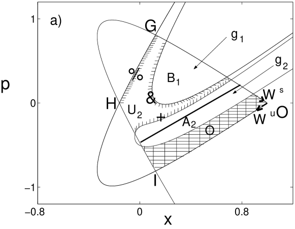
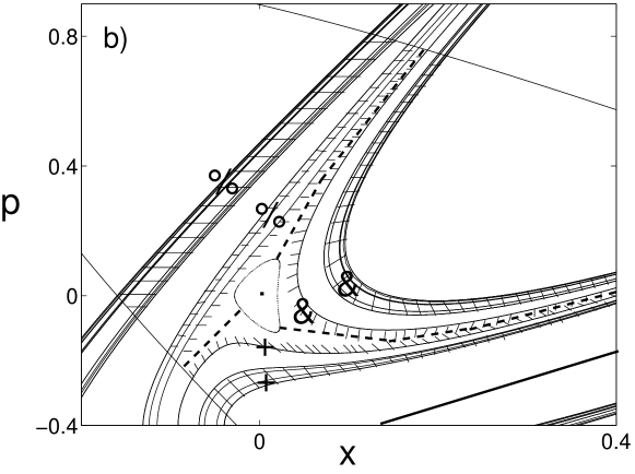
Figure 1:

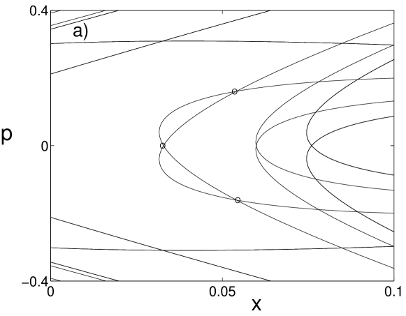
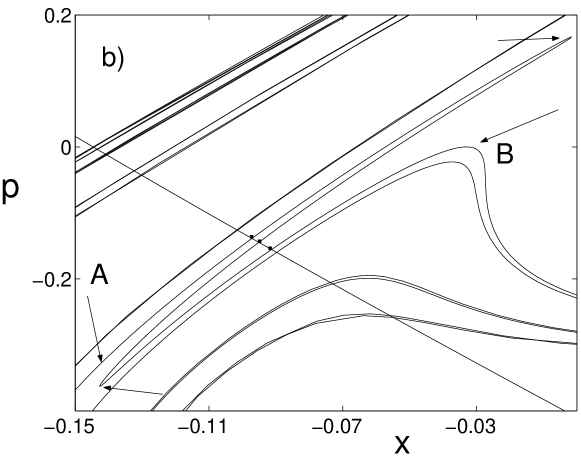
Figure 2:

Figure 3:

Figure 4:

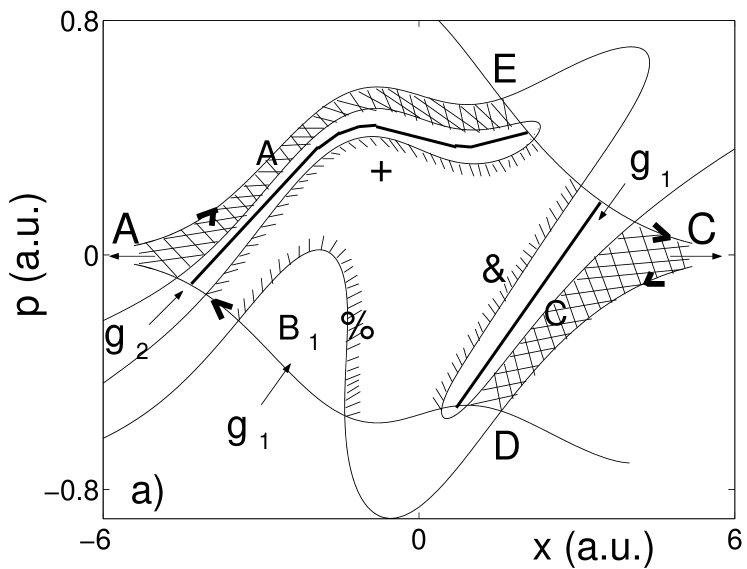
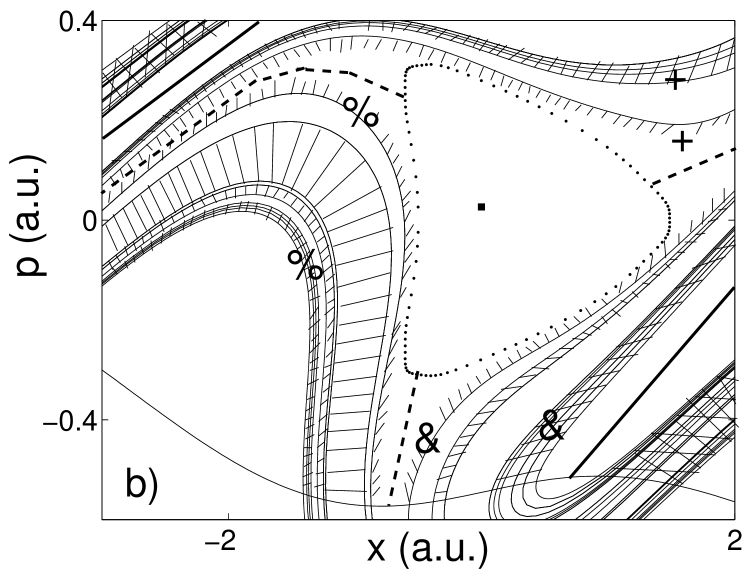
Figure 5:

References

- [1] M. J. Feigenbaum, M. H. Jensen and I. Procaccia, Phys. Rev. Lett. 57, 1503 (1986); C. Beck and F.Schlogel, Thermodynamics of chaotic systems, Cambridge Univ. Press, Cambridge, UK, 1993; G. Karolyi and T. Tl, Physics Reports 290, 125 (1997); B. Rckerl and C. Jung, J. Phys. A. 27, 6741 (1994).
- [2] S. Smale, Bull. Am. Math. Soc. 73, 747 (1967).
- [3] P. Cvitanovic, G. Gunaratne and I. Procaccia, Phys. Rev. A 38, 1503 (1988).
- [4] P. Grassberger and H. Kantz, Phys. Lett. A 113, 235 (1985).
- [5] P. Grassberger, H. Kantz, and U. Moenig, J. Phys. A 22, 5217 (1989).
- [6] K. T. Hansen, Phys. Lett. A 165, 100 (1992).
- [7] F. Giovannini and A. Politi, Phys. Lett. A 161, 332 (1992).
- [8] F. Christiansen and A. Politi, Phys. Rev. E 51 R3811 (1995).
- [9] F. Christiansen and A. Politi, Nonlinearity 9, 1623 (1996).
- [10] C. Lipp and C. Jung, Chaos 9, 706 (1999).
- [11] S. Wiggins, Introduction to Applied Nonlinear Dynamical Systems and Chaos, Springer, 1990.
- [12] B. Rckerl and C. Jung, J. Phys. A. 27, 55 (1994).
- [13] C. Jung, C. Lipp and T. H. Seligman, Annals of Physics 275, 151 (1999).
- [14] H. Tapia and C. Jung, Phys. Lett. A 313, 198 (2003).
- [15] M. Marinescu and M. Gavrila, Phys. Rev. A 53, 2513 (1996); J. N. Bardsley and M. J. Comells, Phys. Rev. A 39, 2252 (1989); A. Emmanouilidou and L. E. Reichl, Phys. Rev. A 65, 33405 (2002).
- [16] H. A. Kramers, Collected Scientific Papers (North-Holland, Amsterdam, 1956), p. 272.
- [17] A. Emmanouilidou, C. Jung and L. E. Reichl, Phys. Rev. E 68, 046207, (2003).
- [18] C. Jung, C. Mejia-Monasterio and T. H. Seligman, Europhys. Lett. 55, 616 (2001).