Thermodynamic formalism for field driven Lorentz gases

Abstract

We analytically determine the dynamical properties of two dimensional field driven Lorentz gases within the thermodynamic formalism. For dilute gases subjected to an iso-kinetic thermostat, we calculate the topological pressure as a function of a temperature-like parameter $\beta$ up to second order in the strength of the applied field. The Kolmogorov-Sinai entropy and the topological entropy can be extracted from a dynamical entropy defined as a Legendre transform of the topological pressure. Our calculations of the Kolmogorov-Sinai entropy exactly agree with previous calculations based on a Lorentz-Boltzmann equation approach. We give analytic results for the topological entropy and calculate the dimension spectrum from the dynamical entropy function.

I Introduction

In dynamical system theory the Lorentz gas acts as a paradigm allowing to address fundamental issues of non-equilibrium processes. Recently, dynamical quantities of this system such as Lyapunov exponents or Kolmogorov-Sinai entropies in a non-equilibrium steady state have been calculated analytically van Beijeren et al. (1996); Latz et al. (1997). Systems like the Lorentz gas in a non-equilibrium steady state can be modeled on the microscopic level by introducing a so-called thermostat which removes the dissipated heat from the system. Assuming that fluids can be regarded as hyperbolic systems on a microscopic level one can relate the dynamical quantities to viscosities or diffusion coefficients Evans and Morriss (1990); Gaspard (1998); Dorfman (1999). This connection is based upon a relation between phase space contraction rates and entropy production.

In the 1960s and 70s Sinai, Ruelle, and Bowen have developed a formalism for dynamical system theory which due to its striking similarity to Gibbs ensemble theory was given the name thermodynamic formalism Sinai (1972); Ruelle (1978); Bowen (1975). This formalism is applied to hyperbolic systems and like in ordinary statistical physics a partition function is defined which is constructed by giving points in phase space a particular weight. From this a central quantity, the topological pressure, is derived which is the dynamical system analog of the Helmholtz free energy. From the dynamical partition function properties like the Kolmogorov-Sinai (KS) entropy or the topological entropy are obtained through the pressure and its derivative with respect to a temperature-like parameter $\beta$. Also derivable are dimension and entropy spectra and, for systems with escape, escape rates.

The paper is organized as follows. In Sec. II we briefly recapitulate some properties of the thermodynamic formalism. Sec. III introduces the field driven Lorentz gas and Sec. IV the concept of the radius of curvature. Calculations for the field driven random Lorentz gas within the thermodynamic formalism in two spacial dimensions are presented in Sec. V. In Sec. VI we calculate dynamical properties from the thermodynamic pressure and we close with some concluding remarks in Sec. VII.

II Thermodynamic formalism

Our starting point is the dynamical partition function, which weighs points in phase space by the local stretching factors $\Lambda(\vec{r},\vec{v},t)$ for trajectory bundles starting at phase space points $(\vec{r},\vec{v})$ and extending over a time $t$. The stretching and contraction factors characterize the behavior of an infinitesimal volume in phase space under the dynamics. Typically, this volume will grow in some directions and shrink in others. Then the local stretching factor is the factor by which the projection of the volume onto its unstable (expanding) directions will increase over time $t$. Similarly, the contraction factor is the factor by which the projection of the same volume onto its stable (contracting) direction is decreased over time $t$. Then, the partition function is defined by

$$Z(\beta,t)=\int{\rm d}\mu(\vec{r},\vec{v})[\Lambda(\vec{r},\vec{v},t)]^{1-\beta},$$ (1)

where a temperature-like parameter $\beta$ is introduced to emphasize the similarity to ordinary statistical physics. The integration is over an appropriate stationary measure.

From Eq.(1) the topological pressure, $P(\beta)$, is obtained as

$$P(\beta)=\lim_{t\rightarrow\infty}\frac{1}{t}\ln Z(\beta,t).$$ (2)

On introducing the Laplace transform ${\cal Z}(\beta,z)\equiv{\cal L}\left\{Z(\beta,t)\right\}$, the calculation of $P(\beta)$ greatly simplifies. From the definition of the Laplace transform we see that ${\cal Z}(\beta,z)$ only converges if $z$ stays smaller than a particular value, the radius of convergence, which is given by $z=\lim_{t\to\infty}\frac{1}{t}\ln Z(\beta,t)=P(\beta)$. Thus, the topological pressure is given by the leading singularity of ${\cal Z}(\beta,z)$, Ruelle (1978).

In analogy to the standard procedures of statistical physics we can define a dynamical entropy function, $h(\beta)$, as the Legendre transform of the topological pressure, i.e.

$$h(\beta)=P(\beta)-\beta\frac{\partial P(\beta)}{\partial\beta}.$$ (3)

For long times the local stretching factors are approximately given by the exponent of the sum of positive Lyapunov exponents, $\lambda_{i}$, multiplied by time, $\Lambda\simeq\exp(t\sum_{i}^{+}\lambda_{i})$. Therefore, it can be shown that the entropy function defined by Eq.(3) can be identified for special values of $\beta$ with dynamical properties. For $\beta=0$, $h(\beta)$ equals the topological entropy, $h_{\rm top}$, whereas for $\beta=1$ it equals the KS entropy, $h_{KS}$ which equals the sum of positive Lyapunov exponents $\sum_{i}^{+}\lambda_{i}$, see for instance Gaspard (1998); Dorfman (1999); Beck and Schlögl (1993).

For systems where trajectories can escape, escape rates can be extracted from the topological pressure. E.g., for $\beta=1$ the topological pressure $P(\beta)$ equals $-\gamma$, where $\gamma$ is the escape rate while the relationship $-\partial P(\beta)/\partial\beta|_{\beta=1}=\sum_{i}^{+}\lambda_{i}$ remains valid. The intersection point of $P(\beta)$ with the $\beta$-axis can be related to the partial Hausdorff dimension, i.e. the fractal dimension of a line across the stable manifold of the attractor (see Gaspard and Baras (1995) for details), while the intersection point of the tangent at $P(1)$ with the $\beta$-axis is associated with the partial information dimension Gaspard and Baras (1995); Bohr and Rand (1987).

III Field driven Lorentz gas

We study the thermodynamic formalism for the dilute, field driven Lorentz gas without escape. This model consists of two species of particles. Heavy, immobile particles of radius $a$ are placed at random positions, while point particles of mass $m$ and charge $q$ move in between them. The interaction between light and heavy particles is modeled by elastic collisions and the heavy particles are not allowed to overlap. An external electric field introduces a force which accelerates the moving particles in the direction of the field and an isokinetic thermostat prevents the system from heating up indefinitely. This thermostat keeps the kinetic energy and thus the speed $v$ of each moving particle constant Evans and Morriss (1990); Hoover (1991). Then, the equations of motions are given by

$$\dot{\vec{r}}=\vec{v}\quad,\qquad\dot{\vec{v}}=\frac{q}{m}\vec{E}-\alpha\vec{v},$$ (4)

where $\alpha=q\vec{E}\cdot\vec{v}/mv^{2}=v_{x}\epsilon/v$, with $\epsilon=qE/mv$. This choice assures that the kinetic energy is kept constant. The electric field is taken to point in the $x$-direction.

Utilizing a Lorentz-Boltzmann equation (LBE) approach Van Beijeren et al. have calculated the Lyapunov spectrum of field-driven dilute Lorentz gases in two and three spacial dimensions van Beijeren et al. (1996); Latz et al. (1997). They did so by extending the usual LBE so as to include the so-called radius of curvature (ROC) tensor, $\boldsymbol{\rho}$, (see Sec. IV). The resulting extended Lorentz-Boltzmann equation (ELBE) for the probability distribution of $\vec{r}$, $\vec{v}$, and $\boldsymbol{\rho}$ reduces to the usual LBE by integrating over $\boldsymbol{\rho}$. From the ELBE the KS entropy is obtained as a steady state ensemble average.

IV Radius of curvature

In order to describe the local stretching factor entering the partition function we have to measure the separation of two nearby trajectories in the course of time. Sinai has given geometric arguments relating this to the ROC Sinai (1970); Gaspard and Dorfman (1995); van Beijeren et al. (1998); Dorfman (1999). Since the light particle moves in $d$ dimensions, and in tangent space the direction of the flow is neither expanding nor contracting, the unstable manifold (the subspace of expanding directions on the energy shell in tangent space) is of dimension $d-1$ (provided the driving field is not too strong). It may be represented by the set of all infinitesimal displacements in position space, orthogonal to the direction of the flow; the stretching factor for large $t$ may be identified with the expansion factor of an infinitesimal volume in this subspace. This expansion factor in turn may be expressed in terms of the ROC.

Figure 1: Illustration of the separation of two nearby trajectories, $\vec{r}(t)$ and $\vec{r}^{\prime}(t)$, for (a) no external field and (b) with an external field, see text for details.

Fig.1 shows a schematic plot of the radius of curvature in two spacial dimensions (in configuration space) in the cases with and without an external field. We measure the separation in a plane perpendicular to the reference trajectory. Let the spacial difference between two trajectories be $\delta\vec{r}(t)$ and the difference in velocity $\delta\vec{v}(t)$ after some time $t$. These vectors satisfy the differential equation

$$\frac{d\delta\vec{r}(t)}{dt}=\delta\vec{v}(t).$$ (5)

The solution of this defines the ROC tensor through the relationship

$$\delta\vec{r}(t)=\frac{1}{v}\boldsymbol{\rho}(t,\delta\vec{r}(0))\cdot\delta\vec{v}(t).$$ (6)

In the absence of external fields, with $\delta\vec{v}$ being constant, the ROC tensor simply is of the form $\boldsymbol{\rho}(t)=vt{\bf 1}+\boldsymbol{\rho}(0)$. Especially in $d=2$, where $\boldsymbol{\rho}$ reduces to a scalar, $\rho(t)$ simply is the distance of the two nearby trajectories to their mutual intersection point, as illustrated in Fig.1. Its sign is positive if the intersection is located in the past and negative if it is in the future.

One sees that already under free streaming the dependence of the ROC on its initial conditions becomes relatively less important as time increases. This is even much more so, if the free streaming is interrupted by collisions. In that case the ROC just before and just after a collision are related in $d=2$ by

$$\rho^{-1}_{+}=\rho^{-1}_{-}+\frac{2}{a\cos\phi},$$ (7)

which may easily be generalized to higher dimensions van Beijeren and Dorfman (2002); Latz et al. (1997). Here $\rho_{-}$ is the pre-collisional ROC, $\rho_{+}$ the ROC directly after the collision, and $\phi$ the angle between the velocity vector at the collision and the outward normal to the scatterer at the point of incidence. Now, the point to notice is that for dilute systems typically $\rho^{-1}_{-}$ is of the order of the inverse mean free path, which is much smaller than the second term on the right hand side of (7). Therefore, to leading order in the density of scatterers this term may be ignored. This implies that the initial value of $\rho$ already gets washed out after one collision. If one cannot use this low density approximation, still a few collisions suffice to make the ROC independent of its initial value. In the sequel of this paper we will use low density approximation, so we set

$$\rho^{-1}_{+}=2/a\cos\phi.$$ (8)

Combining Eqs. (5) and (6) one finds that that the stretching factor over a time $\tau$ now may be expressed in terms of the ROC tensor as

$$\Lambda(\tau)=\exp\left[v\int_{0}^{\tau}{\rm d}t\det(\boldsymbol{\rho}^{-1}(t))\right].$$ (9)

From this the KS entropy may be obtained as

$$h_{KS}=\lim_{t\to\infty}\frac{v}{t}\int\limits_{0}^{t}{\rm d}\tau\det(\boldsymbol{\rho}^{-1}(\tau))=v\left<\det(\boldsymbol{\rho}^{-1})\right>_{\rm stat}.$$ (10)

The bracket $\langle\cdots\rangle_{\rm stat}$ denotes an average over a stationary non-equilibrium distribution on phase space. Its equivalence to a time average requires ergodicity of the motion of the moving particle on the chaotic attractor. About the validity of this even less is known than about ergodicity in equilibrium, in the absence of a driving field. In our calculations we will actually make plausible assumptions about the time average rather than using the phase space average.

For calculating the increase of the stretching factor measured from directly after a collision to directly after the subsequent one, one has to integrate $\det(\boldsymbol{\rho}^{-1}(t))$ over this time interval and insert the result into Eq. (9). For ${\cal{N}}$ uncorrelated collisions taking place over time $t$, the corresponding stretching factor is given by the product of the ${\cal{N}}$ individual stretching factors. The KS entropy is calculated by dividing the logarithm of the stretching factor by $t$ and then taking the long time limit van Beijeren et al. (1998); Latz et al. (1997); Dorfman (1999).

V Thermodynamic formalism for field driven Lorentz gas

In van Beijeren and Dorfman (2002) Van Beijeren and Dorfman present calculations in $d$ dimensions for the dilute random Lorentz gas without an external force. There, the dynamical partition function is calculated by assuming that subsequent collisions are completely uncorrelated. Under this assumption all free times between subsequent collisions may be assumed to be distributed according to the same exponential function and all scattering angles also follow the same simple distribution. In the present case, where the moving particle still has constant speed, we will make the same assumptions, but now the free motion in between collisions is not along straight lines any more.

For simplicity we from now on will restrict ourselves to the case of $d=2$, although the generalization to higher dimensions is fairly straightforward. As in van Beijeren and Dorfman (2002) we divide up the time interval $[0,t]$ into subintervals $[t_{r-1},t_{r}]$, with $t_{r}$ the instant of the $r$-th collision of the moving particle within this time interval. Let the total number of collisions be ${\cal{N}}$, then $t_{0}=0$ and $t_{{\cal{N}}+1}=t$. The total stretching factor can be factorized into a product as

$$\Lambda(t)=\prod_{r=0}^{{\cal{N}}}\Lambda_{r},$$ (11)

where $\Lambda_{r}\equiv\Lambda(\tau_{r})$ is given by Eq.(9), with $\tau_{r}=t_{r-1}-t_{r}$. For obtaining an explicit expression for this we have to solve the differential equation describing the time evolution of the ROC, which is of the form van Beijeren et al. (1996); Latz et al. (1997)

$$\dot{\rho}=v+\rho\epsilon\cos\theta+\rho^{2}\dfrac{\epsilon^{2}}{v}\sin^{2}\theta,$$ (12)

where $\theta$ is the angle between the velocity vector $\vec{v}(t)$ and the external field. As initial condition we will use the low density approximation $\rho_{r_{+}}=a/2\cos\phi_{r}$, with $\phi_{r}$ the collision angle of the $r$th collision. From the equations of motion it follows that $\theta$ obeys the differential equation $\dot{\theta}=-\epsilon\sin\theta$ which has the solution

$$\theta(t,\theta^{+})=\,{\rm arccot}\Big{[}\sinh\big{(}\epsilon t+\kappa\big{)}\Big{]},\quad\kappa=\ln\big{[}\cot(\theta^{+}/2)\big{]}.$$ (13)

Here, $\theta^{+}=\theta(0,\theta^{+}_{r})$ is the angle between the external field and the velocity direction directly after the $r$th collision, compare Fig.1(b). With this solution for $\theta(t)$ we rewrite Eq.(12) as

$$\dot{\rho}=v+\rho\epsilon\tanh(\epsilon t+\kappa)+\rho^{2}\frac{\epsilon^{2}}{v\cosh^{2}(\epsilon t+\kappa)}.$$ (14)

We find for the ROC

$$\rho(t)=\frac{v}{\epsilon}\cosh(\epsilon t+\kappa)\frac{\sinh(\epsilon t+\kappa)-\frac{v\cosh\kappa\sinh\kappa-\epsilon\rho_{+}}{v\cosh\kappa+\epsilon\rho_{+}\sinh\kappa}}{1+\sinh(\epsilon t+\kappa)\frac{v\cosh\kappa\sinh\kappa-\epsilon\rho_{+}}{v\cosh\kappa+\epsilon\rho_{+}\sinh\kappa}}.$$ (15)

Inserting this into Eq.(9) we find, to second order in $\epsilon$,

$$\Lambda_{r} = \Lambda_{r}^{(1)}\Lambda_{r}^{(2)}$$ (16)

$$\Lambda_{r}^{(1)} = \frac{v\tau_{r}}{\rho_{r_{+}}}$$ (17)

$$\Lambda_{r}^{(2)}=\exp\Big{[}-\frac{\epsilon\tau_{r}}{2}\cos\theta^{+}_{r} + \frac{\epsilon^{2}\tau_{r}^{2}}{24}\left(1-9\sin^{2}\theta^{+}_{r}\right)\Big{]}.\quad$$ (18)

Note that the above equations may also be used for $r=0$ but with $\rho_{{}_{0_{+}}}$ and $\theta^{+}_{0}$ given by the initial values of $\rho$ respectively $\theta$ at $t=0$.

For obtaining the topological pressure one has to substitute the above results into Eq.(11), raise this to the power $(1-\beta)$ and average over the configurations of scatterers. For simplifying this average it turns out to be useful to rearrange Eq.(11) as

$$\Lambda(t)=v\tau_{{}_{\cal{N}}}\Lambda_{{}_{\cal{N}}}^{(2)}\left[\prod_{r=1}^{{\cal{N}}}\Gamma_{{}_{{\cal{N}}-r}}\right]\ \rho_{{}_{0_{+}}}^{-1}$$ (19)

where

$$\Gamma_{r}=\Gamma(\tau_{r},\theta^{+}_{r+1},\theta^{+}_{r})\equiv\frac{v\tau_{r}}{\rho_{{}_{(r+1)_{+}}}}\Lambda^{(2)}_{r}.$$ (20)

The reduction to the independent variables implied here follows from Eq.(8) combined with the relationship

$$2\phi_{r}=\theta^{+}_{r}-\theta^{-}_{r}\pm\pi$$ (21)

and $\theta^{-}_{r}$ may be expressed in terms of $\theta^{+}_{r-1}$ and $\tau_{r-1}$ through Eq.(13).

A further simplification can be made by passing to the Laplace transform ${\cal{Z}}(\beta,z)$ of the dynamical partition function. Since, in the limit of large $t$, the topological pressure equals the logarithm of the stretching factor per unit time, it may be identified as the rightmost singularity of this Laplace transform. It has to be real, as the stretching factor is real and positive definite. Assuming independence of all free flight times $\tau_{j}$ and scattering angles $\phi_{j}$ one finds straightforwardly that ${\cal{Z}}(\beta,z)$ may be obtained as

$${\cal{Z}}(\beta,z) = \sum\limits_{{\cal{N}}=0}^{\infty}\int{\rm d}\theta^{+}_{{\cal{N}}}\cdots\int{\rm d}\theta^{+}_{0}\ \hat{\cal M}_{f}(\beta,z,\theta^{+}_{{\cal{N}}})$$ (22)

$$\times\prod\limits_{r=1}^{{\cal{N}}}\hat{{\cal M}}(\beta,z,\theta^{+}_{{\cal{N}}-r+1},\theta^{+}_{{\cal{N}}-r})\ \rho_{{}_{0_{+}}}^{-1}$$

$$= \sum\limits_{{\cal{N}}=0}^{\infty}\left\{\hat{\mathfrak{M}}_{f}\hat{\mathfrak{M}}^{\cal{N}}\ \rho_{{}_{0_{+}}}^{-1}\right\}(\beta,z,\cdot)$$

$$= \left\{\hat{\mathfrak{M}}_{f}\left[{\bf 1}-\hat{\mathfrak{M}}\right]^{-1}\ \rho_{{}_{0_{+}}}^{-1}\right\}(\beta,z,\cdot)\quad$$

Here the operators $\hat{{\cal M}}_{f}$ and $\hat{{\cal M}}$ are defined as the Laplace transforms of the configurational averages of the appropriate powers of $v\tau_{\cal{N}}\Lambda_{\cal{N}}^{(2)}$ and $\Gamma(\tau_{r},\theta_{r+1},\theta_{r})$, respectively. Specifically, one has

$$\hat{{\cal M}}(\beta,z,\theta^{+}{{}^{\prime}},\theta^{+}) = \int\limits_{0}^{\infty}{\rm d}\tau\ \nu\ e^{-(z+\nu)\tau}\int\limits^{\pi/2}_{-\pi/2}{\rm d}\phi\ \frac{\cos\phi}{2}$$ (23)

$$\times\ \delta\left[\phi-\frac{1}{2}\left(\theta^{+}{{}^{\prime}}-\theta(\tau,\theta^{+})\pm\pi\right)\right]$$

$$\times\ \left[\Gamma(\tau,\theta^{+}{{}^{\prime}},\theta^{+})\right]^{1-\beta},$$

$$\hat{\cal M}_{f}(\beta,z,\theta^{+}_{{\cal{N}}}) = V\int\limits_{0}^{\infty}{\rm d}\tau_{\cal{N}}\ \nu\ e^{-(z+\nu)\tau_{\cal{N}}}\left(v\tau_{\cal{N}}\Lambda_{\cal{N}}^{(2)}\right)^{1-\beta}\quad$$ (24)

with $\theta(\tau,\theta^{+})$ defined in Eq.(13). The operators $\hat{\mathfrak{M}}$ and $\hat{\mathfrak{M}}_{f}$ are defined by

$$\left\{\hat{\mathfrak{M}}f\right\}(\beta,z,\theta^{+}{{}^{\prime}}) = \int{\rm d}\theta^{+}\hat{\cal M}(\beta,z,\theta^{+}{{}^{\prime}},\theta^{+})f(\theta^{+})$$ (25)

$$\left\{\hat{\mathfrak{M}}_{f}f\right\}(\beta,z,\cdot) = \int{\rm d}\theta^{+}\hat{\cal M}_{f}(\beta,z,\theta^{+})f(\theta^{+})$$ (26)

where integration limits of the $\theta^{+}$-integrations depend on the sign of $\pi$ in the delta function in Eq.(23) and are given in the Appendix. Further, ${\bf 1}$ denotes the unit operator and $[\cdots]^{-1}$ the operator inverse.

From the above equations the rightmost singularity of ${\cal{Z}}$ readily follows as the value of $z$ for which the largest eigenvalue of the operator $\hat{{\mathfrak{M}}}$ equals unity. For zero field this eigenvalue problem is trivial: the leading eigenfunction is the unit function, the eigenvalue is obtained easily and the resulting topological pressure coincides with that found in van Beijeren and Dorfman (2002). For small non-zero field one has to proceed by expanding $\hat{{\mathfrak{M}}}$, the leading eigenfunction $f$ and the leading eigenvalue $\mu$ in powers of the field strength, i.e.

$$\hat{\mathfrak{M}} = \hat{\mathfrak{M}}^{(0)}+\epsilon\hat{\mathfrak{M}}^{(1)}+\epsilon^{2}\hat{\mathfrak{M}}^{(2)}$$ (27)

$$f = f^{(0)}+\epsilon f^{(1)}+\epsilon^{2}f^{(2)}$$ (28)

$$\mu = \mu^{(0)}+\epsilon\mu^{(1)}+\epsilon^{2}\mu^{(2)}.$$ (29)

Then $\hat{\mathfrak{M}}f=\mu f$ is solved by standard perturbation methods using a Fourier series expansion for $f$, i.e.

$$f^{(i)}=a_{o}^{(i)}+\sum_{n=1}^{\infty}a_{n}^{(i)}\cos(n\theta^{+})+\sum_{n=1}^{\infty}b_{n}^{(i)}\sin(n\theta^{+}),$$ (30)

with $i=0,1,2$.

The details of the solution of this eigenvalue equation are given in the Appendix A. Here we just give the resulting eigenvalue $\mu$ to second order in the field strength,

$$\mu(\beta,z) = \mu^{(0)}(\beta,z)+\epsilon^{2}\mu^{(2)}(\beta,z)$$ (31)

$$= \nu\left(\frac{v}{a}\right)^{1-\beta}\frac{\Gamma\left(\frac{1}{2}\right)\Gamma\left(\frac{\beta+1}{2}\right)\Gamma(2-\beta)}{2^{\beta}\Gamma\left(\frac{\beta}{2}+1\right)(\nu+z)^{2-\beta}}$$

$$\times\Bigg{[}1+\epsilon^{2}\frac{(\beta-1)(\beta-2)(\beta-12)}{48(\nu+z)^{2}}\Bigg{]}.\quad$$

Now the Laplace transform of the dynamical partition function is of the form

$${\cal Z}(\beta,z)=C(\beta,z)\left[1-\mu(\beta,z)\right]^{-1},$$ (32)

where the additional prefactor $C$, originating from $\hat{\mathfrak{M}}(\beta,z,\cdot,\theta^{+}_{{\cal{N}}})$, contains no singularities.

If we also want to obtain information about the contracting direction, e.g. the negative Lyapunov exponents, we need to know the local contraction factors. For this we may consider the time reversed motion. Note, that we will consider the time reversed motion on the attractor for the “forward in time motion” and not the attractor of the time reversed motion. The contraction factors can be calculated by considering contracting trajectory bundles instead of expanding ones van Beijeren et al. (1998), see Fig.2.

Figure 2: Illustration of expanding and contracting trajectory bundles for the two dimensional field driven random Lorentz gas.

We keep the same notation as for the forward in time motion, therefore collision $r$ precedes collision $r-1$ in the time reversed motion. Hence the boundary condition for $\rho(t)$ in Eq.(14) is $\rho(\tau)=\rho_{-}=a\cos\phi/2$, where $\rho_{-}$ specifies the ROC directly before a collision (in the forward in time motion). The ROC still evolves in time according to Eq.(14) for $0\leq t\leq\tau$. Like the expansion factors, one calculates the local contraction factors by using Eq.(9). To second order in $\epsilon$ this yields

$$\Lambda^{-}_{r} = \Lambda_{r}^{(1)-}\Lambda_{r}^{(2)-},$$ (33)

$$\Lambda_{r}^{(1)} = \frac{\rho_{r_{-}}}{v\tau_{r}},$$ (34)

$$\Lambda_{r}^{(2)}=\exp\Big{[}-\frac{\epsilon\tau_{r}}{2}\cos\theta^{+}_{r} + \frac{\epsilon^{2}\tau_{r}^{2}}{24}\left(1+3\sin^{2}\theta^{+}_{r}\right)\Big{]},\qquad$$ (35)

with $\rho_{r_{-}}=a\cos\phi_{r}/2$. In the limit of vanishing external field the contraction factor is just the inverse of the stretching factor. This is no longer true if we apply an external field. We see from Eqs. (18) and (35) that differences occur in the field dependent exponential.

To obtain a topological pressure for the contracting directions we have to solve a similar eigenvalue problem as for the expanding directions. Since for the field free case the inverse of the contraction factor equals the stretching factor, we solve the eigenvalue problem for the inverse of the contraction factor. The resulting eigenvalue, which has to be set equal to unity again, to second order in field strength becomes

$$\mu^{-}(\beta,z) = \nu\left(\frac{v}{a}\right)^{1-\beta}\frac{\Gamma\left(\frac{1}{2}\right)\Gamma\left(\frac{\beta+1}{2}\right)\Gamma(2-\beta)}{2^{\beta}\Gamma\left(\frac{\beta}{2}+1\right)(\nu+z)^{2-\beta}}$$ (36)

$$\times\Big{[}1-\epsilon^{2}\frac{(\beta-1)(\beta-2)(\beta-8)}{48(\nu+z)^{2}}\Big{]}.$$

Details are given again in the Appendix A.

In the following section we will discuss the resulting topological pressure and related properties.

VI Dynamical properties

As stated in the preceding section the topological pressure follows as the value of $z$ for which $\mu(\beta,z)=1$. To second order in $\epsilon$ this leads to

$$P(\beta)=P_{0}(\beta)-\epsilon^{2}\frac{(\beta-1)(\beta-12)}{48(P_{0}(\beta)+\nu)}$$ (37)

where

$$P_{0}(\beta)=\left[\frac{\nu}{2}\Big{(}\frac{v}{a}\Big{)}^{(1-\beta)}\ \frac{\Gamma(2-\beta)\Gamma\left(\frac{1}{2}\right)\Gamma\left(\frac{\beta+1}{2}\right)}{2^{\beta}\Gamma\left(\frac{\beta}{2}+1\right)}\right]^{\frac{1}{2-\beta}}-\nu$$ (38)

is the field free value of the topological pressure. The dynamical entropy then follows from Eq.(3) as

$$h(\beta) = P(\beta)-\beta\frac{\partial P(\beta)}{\partial\beta}$$ (39)

$$= h_{0}(\beta)-\frac{\epsilon^{2}}{48(P_{0}(\beta)+\nu)}\Bigg{[}12-\beta^{2}$$

$$+\frac{\beta(\beta-1)(\beta-12)}{P_{0}(\beta)+\nu}\cdot\frac{\partial P_{0}(\beta)}{\partial\beta}\Bigg{]}$$

where again $h_{0}(\beta)$ is the field free value of the dynamical entropy.

We can perform similar calculations for the contracting direction. Then we obtain the equivalent of the topological pressure and the dynamical entropy. Note that in the limit of vanishing external field the topological pressure for the contracting direction equals the one for the expanding direction. We obtain

$$P^{-}(\beta) = P_{0}(\beta)+\epsilon^{2}\frac{(\beta-1)(\beta-8)}{48(P_{0}(\beta)+\nu)}$$ (40)

$$h^{-}(\beta) = h_{0}(\beta)+\frac{\epsilon^{2}}{48(P_{0}(\beta)+\nu)}\Bigg{[}8-\beta^{2}$$ (41)

$$+\frac{\beta(\beta-1)(\beta-8)}{P_{0}(\beta)+\nu}\cdot\frac{\partial P_{0}(\beta)}{\partial\beta}\Bigg{]}.$$

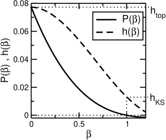
Figure 3: The topological pressure, $P(\beta)$, and the dynamical entropy, $h(\beta)$, for small fields and small densities of scatterers, i.e. $\epsilon=0.001,\ n=0.001,\ v=1,\ a=1$.

Fig.3 shows the topological pressure and the dynamical entropy as functions of the parameter $\beta$. As expected for a system without escape, $P(\beta)$ vanishes for $\beta=1$. We further see that $P(\beta)$ is a convex function.

A number of interesting dynamical quantities are related to the dynamical entropy, $h(\beta)$, for special values of $\beta$. The KS entropy, $h_{KS}$, is given by the dynamical entropy for $\beta=1$. From Eq.(39) we obtain

$$h_{KS}=\lambda^{+}=\nu\left(1-\gamma-\ln\left(\frac{a\nu}{v}\right)\right)-\frac{11}{48}\frac{\epsilon^{2}}{\nu}.$$ (42)

For the negative Lyapunov exponent we yield, from Eq.(41)

$$-h^{-}(1)=\lambda^{-}=-\nu\left(1-\gamma-\ln\left(\frac{a\nu}{v}\right)\right)-\frac{7}{48}\frac{\epsilon^{2}}{\nu}.$$ (43)

As one should expect, these results coincide with those of previous calculations van Beijeren et al. (1996); Latz et al. (1997) based on the same assumptions (basically, no correlations between subsequent collisions). But here the results are extended to general values of $\beta$.

New results follow for the topological entropy, which is given by the dynamical entropy for $\beta=0$. From Eq.(39) we obtain

$$h_{\rm top}=\left[\frac{\pi\nu v}{a}\right]^{\frac{1}{2}}-\nu-\frac{\epsilon^{2}}{4}\left[\frac{a}{\pi\nu v}\right]^{\frac{1}{2}}$$ (44)

That is, we obtain the zero field limit results given in van Beijeren and Dorfman (2002) with a correction which is quadratic in the field strength.

The equivalend of the topological entropy for the contracting direction is obtained from Eq.(41) for $\beta=0$, i.e.

$$h^{-}(0)=\left[\frac{\pi\nu v}{a}\right]^{\frac{1}{2}}-\nu+\frac{\epsilon^{2}}{6}\left[\frac{a}{\pi\nu v}\right]^{\frac{1}{2}}.$$ (45)

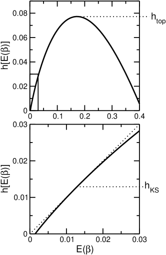
Figure 4: Dynamical entropy, $h[E(\beta)]$, as a function of $E(\beta)=-\partial P(\beta)/\partial\beta$ for $\epsilon=0.001$, $n=0.001$, $a=1$, and $v=1$. The lower panel is a close-up of the boxed region of the upper panel.

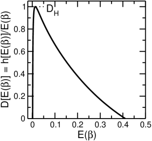
Figure 5: Dimension spectrum for $\epsilon=0.001$, $n=0.001$, $a=1$, and $v=1$. The maximum occurs for $\beta=1$.

We further calculate the dynamical entropy as a function of $E(\beta)\equiv-\partial P(\beta)/\partial\beta$, Bohr and Rand (1987). $E(\beta)$ equals the average of the logarithm of the local stretching factors, $\left<\ln\Lambda\right>_{\beta}$, where the subscript $\beta$ refers to the fact that in phase space initial points are weighted according to the stretching factors raised to the power $(1-\beta)$. For $\beta=1$ this yields the average of the positive Lyapunov exponent.

The maximum entropy, which is the topological entropy, is always found for $\beta=0$ as can be seen from Eq.(3). The KS entropy is given by the value for $\beta=1$ where $h[E(\beta)]=E(\beta)$, again according to Eq.(3). In Fig.4 a plot of $h[E(\beta)]$ vs. $E(\beta)$ is given. But notice that the descending parts of $h[E(\beta])$ correspond to values of $\beta\leq 0$.

The dynamical entropy is related to a dimension spectrum, $D(\alpha)$, with $\alpha=E(\beta)$, through $D(\alpha)=h(\alpha)/\alpha$ Bohr and Rand (1987). Fig.5 shows the dimension spectrum, $D[E(\beta)]$. From this one can find the partial Hausdorff dimension, $D_{H}$, as the maximum of $D[E(\beta)]$. For systems where trajectories cannot escape, $D_{H}$ equals one. This is clear because the maximum of $D[E(\beta)]$ is obtained for $P(\beta)=0$, i.e. $\beta=1$, for systems without escape. Note that possible values of partial dimensions are restricted to the interval $[0,1]$, see Sec.II. Furthermore, the full Hausdorff dimension is $D_{H}^{\rm full}\leq\sum_{i=1}^{3}D_{H}^{(i)}$ where the $D_{H}^{(i)}$ are the partial Hausdorff dimensions corresponding to all stable and unstable manifolds Eckmann and Ruelle (1985).

The above results for the dynamical entropy allow to calculate, respectively approximate, another dimension, the Kaplan-Yorke dimension, $D_{KY}$. In general the Kaplan-Yorke dimension is given by $D_{KY}=n+\sum_{i=1}^{n}\lambda_{i}/|\lambda_{n+1}|$ where $n$ is given by the largest value for which $\sum_{i=1}^{n}\lambda_{i}\geq 0$. Thus for the two dimensional Lorentz gas with constant energy we have one exponent equal to $0$, one positive, and one negative, i.e. we have $D_{KY}=2+\lambda^{+}/|\lambda^{-}|$. There are only three exponents since the system is restricted to a three dimensional hyperplane by the thermostat. From the KS entropies we see that $D_{KY}\approx 3-3\epsilon^{2}/(8h_{KS}^{0}\nu)$, where $h_{KS}^{0}$ is the KS entropy without external field. Since the exact full Hausdorff dimension and therefore also the full information dimension cannot be extracted from the partial dimensions we assume that the Kaplan-Yorke conjecture still holds. This is consistent with our present knowledge: because $D_{H}^{\rm full}\leq\sum_{i=1}^{3}D_{H}^{(i)}=3$ we still can have $D_{H}^{\rm full}=D_{KY}$. Let us further mention that the dimensional loss due to the external field, as expressed by $D_{KY}$, is rather small in the region where the above results hold, i.e. for small fields and low densities, see also Evans et al. (2000).

The calculated dynamical properties allow for the extraction of macroscopic transport coefficients. The diffusion coefficient is given by ${\cal D}=-\lim_{\epsilon\to 0}[v^{2}(\lambda_{+}(\epsilon)+\lambda_{-}(\epsilon))]\epsilon^{-2}=(3/8)v^{2}/\nu$, van Beijeren et al. (1996), which can also be expressed in terms of the Kaplan-Yorke dimension by ${\cal D}=-\lim_{\epsilon\to 0}[v^{2}h^{0}_{KS}(D_{KY}-3)]\epsilon^{-2}$, Evans et al. (2000).

Some comment on the calculations of the topological pressure as a function of the temperature-like parameter $\beta$ is in order here. The obtained results have to be taken with a pinch of salt. In van Beijeren and Dorfman (2002) and Appert et al. (1996) it is shown that for the random Lorentz gas the results obtained there are restricted to increasingly smaller neighborhoods of $\beta\approx 1$ for increasing system size. As can be seen from Eq.(1), for $\beta=1$ all points in phase space are equally weighted. For $\beta<1$, though, the partition function will be dominated by the largest stretching factors, which correspond to the most unstable trajectory bundles. That is, for $\beta<1$ stretching factors from regions in phase space with a high density of scatterers, and therefore large stretching factors, dominate. So, in the limit $t\to\infty$ it is possible that $Z(\beta,t)$ is dominated by trajectory bundles confined to a small part of phase space. In regions of high scatterer density however, subsequent scattering events cannot be regarded as independent any more and the distribution of free times between scatterers in these regions will be very different from that for the system as a whole. With increasing system size the effects become more pronounced because the probability of finding approximately trapping regions of high scatterer density increases with system size.

VII Conclusion

In the present study we have calculated dynamical properties for the field driven random Lorentz gas within the thermodynamic formalism. In the limits of vanishing external field or $\beta$ approaching unity, our results are in perfect agreement with those of previous studies.

From the topological pressure we extracted various quantities, such as the KS entropy and the topological entropy. A dimension spectrum was obtained by calculating the dynamical entropy as a function of the variable $E(\beta)$, defined as the derivative with respect to $\beta$ of the topological pressure.

Van Beijeren and Dorfman have calculated KS entropies and topological entropies for general dimensions $d$ for the random Lorentz gas without an external field van Beijeren and Dorfman (2002). Presently we work on the extension of the present study to higher dimensions. Subtleties exist because an external field complicates the analytic calculation of the determinant of the inverse of the ROC tensor for higher dimensions quite a bit. However, the stretching factors can also be calculated by looking at the time evolution of the deviations in velocity, see van Beijeren et al. (1998).

We also extended our studies to systems with open boundaries Mülken and van Beijeren (2003). This allows for using the thermodynamic formalism to study the escape rate formalism Gaspard and Nicolis (1990), as well as dimension spectra for systems with escape. In the limit of $\beta\to 1$ comparison can be made again with previous results van Beijeren et al. (2000).

*

Appendix A Calculation of the dynamical partition function

Starting with the dynamical partition function we can determine the topological pressure which is given as the leading singularity of the Laplace transform of the dynamical partition function.

In order to calculate the Laplace transform of the dynamical partition function, Eq.(22), we need to calculate the eigenfunctions and eigenvalues of $\hat{\mathfrak{M}}$. According to Eq.(27) we expand $\hat{\mathfrak{M}}$ in powers of $\epsilon$, yielding

$$\hat{\mathfrak{M}}(\beta,z,\theta^{+}{{}^{\prime}}) = \int\limits_{0}^{\infty}{\rm d}\tau\int\limits_{-\pi/2}^{\pi/2}{\rm d}\phi\int{\rm d}\theta^{+}\ \nu\ e^{-(\nu+z)\tau}\ \frac{\cos\phi}{2}\ \delta\left[\phi-\frac{1}{2}(\theta^{+}{{}^{\prime}}-\theta(\tau,\theta^{+})\pm\pi\right]\left[\frac{2v\tau}{a\cos\phi}\right]^{1-\beta}$$ (46)

$$\times\left\{1-\epsilon\frac{\tau}{2}\cos\theta^{+}+\epsilon^{2}\frac{\tau^{2}}{24}\left[1-9\sin\theta^{+}+3\cos^{2}\theta^{+}\right]\right\}^{1-\beta},$$

The operator $\hat{\mathfrak{M}}$ has to be understood as acting on a function $f(\theta^{+})$. In order to eliminate the $\delta$-function we integrate over $\theta^{+}$ first by noticing that we can write $\delta[g(\theta^{+})]=\delta(\theta^{+}-\theta^{+}_{0})/g^{\prime}(\theta^{+}_{0})$ where $\theta^{+}_{0}$ is the root of $g(\theta^{+}_{0})$ and the prime denotes the derivative with respect to $\theta^{+}$. Here we have

$$g^{\prime}(\theta^{+}_{0})=\frac{1}{2}-\frac{\epsilon\tau}{2}\cos\theta^{+}_{0}+\frac{(\epsilon\tau)^{2}}{4}\cos(2\theta^{+}_{0})$$ (47)

with

$$\theta^{+}_{0}=\theta^{+}{{}^{\prime}}-2\phi+\epsilon\tau\sin\theta^{+}_{0}-\frac{(\epsilon\tau)^{2}}{4}\sin(2\theta^{+}_{0})\pm\pi.$$ (48)

Then the operator $\hat{\mathfrak{M}}(\beta,z,\theta^{+}{{}^{\prime}})$ becomes

$$\hat{\mathfrak{M}}(\beta,z,\theta^{+}{{}^{\prime}}) = \int\limits_{0}^{\infty}{\rm d}\tau\int\limits_{-\pi/2}^{\pi/2}{\rm d}\phi\ \nu\ e^{-(\nu+z)\tau}\ \frac{\cos\phi}{2}\left[\frac{2v\tau}{a\cos\phi}\right]^{1-\beta}2\left(1+\epsilon\tau\cos\theta^{+}_{0}+\frac{(\epsilon\tau)^{2}}{2}\right)$$ (49)

$$\times\left\{1-\epsilon\frac{\tau}{2}\cos\theta^{+}+\epsilon^{2}\frac{\tau^{2}}{24}\left[-2+6\cos(2\theta^{+})\right]\right\}^{1-\beta}$$

This is expanded to second order and the operator $\hat{\mathfrak{M}}$ acting on $f(\theta^{+})$ then reads

$$\hat{\mathfrak{M}}f(\theta^{+})=\left[\hat{\mathfrak{M}}f\right](\theta^{+}{{}^{\prime}})=\left[\hat{\mathfrak{M}}^{(0)}f\right](\theta^{+}{{}^{\prime}})+\epsilon\left[\hat{\mathfrak{M}}^{(1)}f\right](\theta^{+}{{}^{\prime}})+\left[\epsilon^{2}\hat{\mathfrak{M}}^{(2)}f\right](\theta^{+}{{}^{\prime}})$$ (50)

$$\mbox{with}\quad\left[\hat{\mathfrak{M}}^{(0)}f\right](\theta^{+}{{}^{\prime}}) = \int\limits_{0}^{\infty}{\rm d}\tau\int\limits_{-\pi/2}^{\pi/2}{\rm d}\phi\ \nu\ e^{-(\nu+z)\tau}\ \left[\frac{2v\tau}{a}\right]^{1-\beta}\cos^{\beta}\phi\ f(\theta^{+}_{0})$$ (51)

$$\left[\hat{\mathfrak{M}}^{(1)}f\right](\theta^{+}{{}^{\prime}}) = -\int\limits_{0}^{\infty}{\rm d}\tau\int\limits_{-\pi/2}^{\pi/2}{\rm d}\phi\ \nu\ e^{-(\nu+z)\tau}\ \left[\frac{2v\tau}{a}\right]^{1-\beta}\cos^{\beta}\phi\ \frac{\tau}{2}(1+\beta)\cos\theta^{+}_{0}\ f(\theta^{+}_{0})$$ (52)

$$\left[\hat{\mathfrak{M}}^{(2)}f\right](\theta^{+}{{}^{\prime}}) = \int\limits_{0}^{\infty}{\rm d}\tau\int\limits_{-\pi/2}^{\pi/2}{\rm d}\phi\ \nu\ e^{-(\nu+z)\tau}\ \left[\frac{2v\tau}{a}\right]^{1-\beta}\cos^{\beta}\phi$$ (53)

$$\quad\times\frac{\tau^{2}}{2}\left(\frac{3\beta^{2}+13\beta+8}{24}+\frac{\beta(\beta-1)}{8}\cos(2\theta^{+}_{0})\right)\ f(\theta^{+}_{0})$$

For small $\epsilon$ we can expand $\cos\theta^{+}_{0}$ and $\cos(2\theta^{+}_{0})$ which gives

$$\cos\theta^{+}_{0} = \cos[\theta^{+}{{}^{\prime}}-2\phi\pm\pi+\epsilon\tau\sin(\theta^{+}{{}^{\prime}}-2\phi\pm\pi)]$$ (54)

$$\approx -\cos(\theta^{+}{{}^{\prime}}-2\phi)-\epsilon\tau\sin^{2}(\theta^{+}{{}^{\prime}}-2\phi)$$

and

$$\cos(2\theta^{+}_{0})\approx\cos(2\theta^{+}{{}^{\prime}}-4\phi).$$ (55)

Since we expand only to second order in $\epsilon$ it is sufficient to expand $\cos\theta^{+}_{0}$ to first order because it only enters in the $\epsilon$-term of Eq.(50). Accordingly, we only take the zeroth order term of $\cos(2\theta^{+}_{0})$. Now the eigenvalues $\mu$ and eigenfunctions $f$ can be calculated by using standard perturbation theory and a Fourier series expansion for $f$ as given in Eq.(30). To zeroth order in $\epsilon$ we find that $f^{(0)}(\theta^{+})={\rm constant}$, which we set equal to $1$. For the eigenvalue we get

$$\mu^{(0)}=\nu\Big{(}\frac{v}{a}\Big{)}^{(1-\beta)}\ \frac{\Gamma(2-\beta)\Gamma\left(\frac{1}{2}\right)\Gamma\left(\frac{\beta+1}{2}\right)}{2^{\beta}(\nu+z)^{2-\beta}\Gamma\left(\frac{\beta}{2}+1\right)}.$$ (56)

Inserting these results into Eq.(52) we get

$$\mu^{(1)} = 0$$ (57)

$$\mbox{and}\quad f^{(1)}(\theta^{+}) = -\frac{\beta(2-\beta)}{4(\nu+z)}\cos\theta^{+}.$$ (58)

The procedure for the $\epsilon^{2}$-terms is analogous. However, when calculating the eigenvalue $\mu^{(2)}$ one finds an additional contribution from $\left[\hat{\mathfrak{M}}^{(0)}f^{(1)}\right](\theta^{+}{{}^{\prime}})$, which also has to be taken into account. This is because of the $\epsilon$-dependent term in Eq.(54). Then to second order in $\epsilon$ the eigenvalue is given by

$$\mu^{(2)}=\mu^{(0)}\frac{(\beta-1)(\beta-2)(\beta-12)}{48(\nu+z)^{2}}$$ (59)

In principle the eigenfunction $f^{(2)}(\theta^{+})$ can be calculated and will be proportional to $\cos(2\theta^{+})$. However, for our results we do not need $f^{(2)}(\theta^{+})$ since the only terms entering in Eq.(31) are $\mu^{(0)}f^{(0)}(\theta^{+})$ and $\epsilon^{2}\mu^{(2)}f^{(0)}(\theta^{+})$.

An analogous calculation for the contracting direction yields for the eigenvalues

$$\bar{\mu}^{(0)} = \nu\Big{(}\frac{v}{a}\Big{)}^{(1-\beta)}\ \frac{\Gamma(2-\beta)\Gamma\left(\frac{1}{2}\right)\Gamma\left(\frac{\beta+1}{2}\right)}{2^{\beta}(\nu+z)^{2-\beta}\Gamma\left(\frac{\beta}{2}+1\right)}$$ (60)

$$\bar{\mu}^{(1)} = 0$$ (61)

$$\bar{\mu}^{(2)} = -\bar{\mu}^{(0)}\frac{(\beta-1)(\beta-2)(\beta-8)}{48(\nu+z)^{2}}$$ (62)

and for the eigenfunctions

$$\bar{f}^{(0)}(\theta^{+}) = 1$$ (63)

$$\bar{f}^{(1)}(\theta^{+}) = -\frac{\beta(2-\beta)}{4(\nu+z)}\cos\theta^{+},$$ (64)

where the bar is indicating the contracting direction. Again, for Eq.(36) we only need the eigenfunctions up to first order in $\epsilon$.

References

- van Beijeren et al. (1996) H. van Beijeren, J. R. Dorfman, E. G. D. Cohen, H. A. Posch, and C. Dellago, Phys. Rev. Lett. 77, 1974 (1996).
- Latz et al. (1997) A. Latz, H. van Beijeren, and J. R. Dorfman, Phys. Rev. Lett. 78, 207 (1997).
- Evans and Morriss (1990) D. J. Evans and G. P. Morriss, Statistical Mechanics of Nonequilibrium Liquids (Academic Press, London, 1990).
- Gaspard (1998) P. Gaspard, Chaos, Scattering, and Statistical Mechanics (Cambridge University Press, Cambridge UK, 1998).
- Dorfman (1999) J. R. Dorfman, An Introduction to Chaos in Non-Equilibrium Statistical Mechanics (Cambridge University Press, New York, 1999).
- Sinai (1972) Y. G. Sinai, Russ. Math. Surv. 27, 21 (1972).
- Ruelle (1978) D. Ruelle, Thermodynamic Formalism (Addison-Wesley Publishing Co., New York, 1978).
- Bowen (1975) R. Bowen, in Lecture Notes in Mathematics (Springer Verlag, Berlin, 1975), vol. 470.
- Beck and Schlögl (1993) C. Beck and F. Schlögl, Thermodynamics of chaotic systems (Cambridge University Press, New York, 1993).
- Gaspard and Baras (1995) P. Gaspard and F. Baras, Phys. Rev. E 51, 5332 (1995).
- Bohr and Rand (1987) T. Bohr and D. Rand, Physica D 25, 387 (1987).
- Hoover (1991) W. G. Hoover, Computational Statistical Mechanics (Elsevier Publ. Co., Amsterdam, 1991).
- Gaspard and Dorfman (1995) P. Gaspard and J. R. Dorfman, Phys. Rev. E 52, 3525 (1995).
- van Beijeren et al. (1998) H. van Beijeren, A. Latz, and J. R. Dorfman, Phys. Rev. E 57, 4077 (1998).
- Sinai (1970) Y. G. Sinai, Russ. Math. Surv. 25, 137 (1970).
- van Beijeren and Dorfman (2002) H. van Beijeren and J. R. Dorfman, J. Stat. Phys. 108, 767 (2002).
- van Beijeren et al. (2000) H. van Beijeren, A. Latz, and J. R. Dorfman, Phys. Rev. E 63, 016312 (2000).
- Eckmann and Ruelle (1985) J.-P. Eckmann and D. Ruelle, Rev. Mod. Phys. 57, 617 (1985).
- Evans et al. (2000) D. J. Evans, E. G. D. Cohen, D. J. Searles, and F. Bonetto, J. Stat. Phys. 101, 17 (2000).
- Appert et al. (1996) C. Appert, H. van Beijeren, M. H. Ernst, and J. R. Dorfman, Phys. Rev. Lett. 54, 54 (1996).
- Mülken and van Beijeren (2003) O. Mülken and H. van Beijeren, unpublished.
- Gaspard and Nicolis (1990) P. Gaspard and G. Nicolis, Phys. Rev. Lett. 65, 1693 (1990).