Soliton on a Cnoidal Wave Background

in the coupled nonlinear Schrödinger equation

H. J. Shin

Department of Physics and Research Institute of Basic Science

Kyung Hee University, Seoul 130-701, Korea

ABSTRACT

An application of the Darboux transformation on a cnoidal wave background in the coupled nonlinear Schrödinger equation gives a new solution which describes a soliton moving on a cnoidal wave. This is a generalized version of the previously known soliton solutions of dark-bright pair. Here a dark soliton resides on a cnoidal wave instead of on a constant background. It also exhibits a new types of soliton solution in a self-focusing medium, which describes a breakup of a generalized dark-bright pair into another generalized dark-bright pair and an “oscillating” soliton. We calculate the shift of the crest of the cnoidal wave along a soliton and the moving direction of the soliton on a cnoidal wave.

1 Introduction

In this paper, we consider a system of coupled nonlinear Schrödinger (CNLS) equations [1, 2, 3]

$$\partial_{\bar{z}}\psi_{k}=-i\partial_{z}^{2}\psi_{k}-2i\sigma(|\psi_{1}|^{2}+|\psi_{2}|^{2})\psi_{k}~{};~{}k=1,2.$$ (1)

These equations, which were named as the Manakov model, are important for a number of physical applications like multi-frequency and/or two different polarizations of light in a fiber [4, 5, 6]. Nowadays, there exist vast amount of exact solutions of this system including exact vector solitons [1, 5], bound solitary waves [7], and periodic solutions [7, 8, 9, 10]. Especially, quasi-periodic solutions in terms of N-phase theta functions for the Manakov model are derived in [11], while a series of special solutions are given in [12, 13, 14, 15].

Recently, this equation attracts new attention as it can describe the localized states in optically induced refractive index gratings [16, 17, 18]. Strong incoherent interaction of such a grating with a probe beam facilitates the formation of a noble type of a composite optical soliton, where one of the components (described by $\psi_{1}$ in Eq. (1)) creates periodic photonic structure, while the other component ($\psi_{2}$) experiences Bragg reflection from this structure and forms gap solitons. Optically induced lattices are very exciting development which open up creating dynamically reconfigurable photonic structures. It was shown that the CNLS equation describes the propagation of two incoherently interacting beams in a photorefractive crystal in the limit of weak saturation regime [19, 18].

To analyze the behavior of the soliton in the optically induced lattices, we need a solution of the CNLS equation that describes a soliton moving on a cnoidal wave. The integrability of the CNLS equation shown by Manakov provides us to obtain various type of solutions. Especially, one can obtain the bright soliton in a focusing medium by applying the inverse scattering method (ISM) [20]. On the other hand, in the case of nonvanishing background fields, the inverse scattering method is technically highly involved and only the dark solitons of the simplest one-component case have been found in this way. In the two component case, the Hirota method has been adopted to obtain dark solitons instead of the ISM [21, 22]. The Hirota method, however, does not provide a way to construct a soliton solution moving on a cnoidal wave background. Interestingly, the (soliton + cnoidal wave) solution can be obtained from the general quasi-periodic solutions of N-phase theta functions, by taking degenerate limit of the 2-phase solution. In fact, Ref. [23] applied this procedure to obtain a solution of the single-component nonlinear Schrödinger equation (NLSE). But solutions from the N-phase theta functions have the so-called “effectivization” problem, which is related to extracting the physical solutions by taking proper initial conditions [24, 10]. Much more, these solutions have rather complicated form, which makes them difficult to apply to real situations.

In this paper, we employ a simple, but very powerful soliton finding technique based on the Darboux transformation (DT). This method is essentially equivalent to the ISM, but avoids mathematical technicalities of the ISM. Section 2 introduces the main method including the DT and Sym’s solution. Section 3 analyzes the characteristics of obtained solutions in the case of focusing medium. Section 4 is devoted to the case of defocusing medium. Section 5 contains a short discussion and Appendices give some proofs of equations in the main text.

2 The Method

2.1 Lax Pair

We first bring the CNLS equation into a matrix form in terms of $3\times 3$ matrices $E,T$ and $\tilde{E}=[T,~{}E]$,

$$E=\pmatrix{0&\psi_{1}&\psi_{2}\cr-\sigma\psi_{1}^{*}&0&0\cr-\sigma\psi_{2}^{*}&0&0},~{}~{}~{}T=\pmatrix{i/2&0&0\cr 0&-i/2&0\cr 0&0&-i/2},$$ (2)

such that

$$\partial_{\bar{z}}E=-\partial_{z}^{2}\tilde{E}+2E^{2}\tilde{E}.$$ (3)

One can readily check that the components of Eq. (3) are indeed equivalent to the Manakov equation in Eq. (1). The signature $\sigma$ is either $1$ or $-1$ depending on whether the group velocity dispersion is abnormal ($\sigma=1$) or normal ($\sigma=-1$), or the waveguide is self-focusing ($\sigma=1$) or self-defocusing($\sigma=-1)$. One advantage of using matrices is that we can write down the associated linear equation (Lax pair);

$$(\partial_{z}+E+\lambda T)\Psi=0,~{}~{}(\partial_{\bar{z}}+E\tilde{E}-\partial_{z}\tilde{E}-\lambda E-\lambda^{2}T)\Psi=0,$$ (4)

where $\lambda$ is an arbitrary complex number and $\Psi(z,\bar{z},\lambda)$ is a three component vector.

2.2 Darboux Transformation

The following cnoidal wave solution of the CNLS equation properly describes the background periodic wave in optically induced refractive index gratings. For the case of focusing medium ($\sigma=1$), it is

$$\psi_{1}^{c}(z,\bar{z})=p~{}{\rm dn}(\chi,k)e^{i\zeta},~{}\psi_{2}^{c}=0,$$ (5)

where $\chi=-p(z-v\bar{z}),~{}\zeta=[-vz/2-p^{2}(2-k^{2})\bar{z}+v^{2}\bar{z}/4]$. The defocusing case ($\sigma=-1$) is obtained by substituting $p\rightarrow ip,k\rightarrow ik$ in Eq. (5) of the focusing case. Here dn, sn is the standard Jacobi elliptic function. And $v$ is the velocity of the cnoidal wave and $k\in(0,1)$ is the modulus of the Jacobi function. As far as elliptic functions are involved we employ terminology and notation of Ref. [25] without further explanations. To describe the characteristics of the composite optical soliton formed on the background grating, we need a soliton solution superposed on the cnoidal wave. To obtain a superposed solution of (soliton + cnoidal wave) using the Darboux transformation, we need to find a solution of the linear equations (4) with $\psi_{i},i=1,2$ given by Eq. (5). We denote the solution of the linear equation as a three component vector, $\Psi=\pmatrix{s_{0}\cr s_{1}\cr s_{2}}$. Then a new solution of (soliton + cnoidal wave) is constructed using the Darboux transformation [26, 27, 28], which is

$$\psi_{i}^{c-s}(z,\bar{z})=\psi_{i}^{c}(z,\bar{z})+i(\lambda-\lambda^{*}){\sigma s_{0}s_{i}^{*}\over|s_{0}|^{2}+\sigma\sum_{j=1,2}|s_{j}|^{2}},~{}i=1,2.$$ (6)

Using that $s_{i}$ satisfy the associated linear equations in Eq. (4), it can be directly checked that $\psi_{i}^{c-s},~{}i=1,2$ in Eq. (6) is a new solution of the CNLS equation.

2.3 Sym’s Solution

Explicitly, the solution of the linear equations in Eq. (4) for $\sigma=1$ can be written down as

$$s_{0} = e^{i\zeta/2}[Me^{i\Delta}\theta_{2}({-iu\over 2K})\theta_{0}({\chi+iu\over 2K})-Ne^{-i\Delta}\theta_{1}({-iu\over 2K})\theta_{3}({\chi-iu\over 2K})]/\theta_{0}({\chi\over 2K}),$$

$$s_{1} = e^{-i\zeta/2}[-Me^{i\Delta}\theta_{1}({-iu\over 2K})\theta_{3}({\chi+iu\over 2K})+Ne^{-i\Delta}\theta_{2}({-iu\over 2K})\theta_{0}({\chi-iu\over 2K})]/\theta_{0}({\chi\over 2K}),$$

$$s_{2} = Ce^{i\lambda z/2-i\lambda^{2}\bar{z}/2},$$ (7)

where $M,N,C$ are arbitrary complex numbers and $\Delta=-\gamma\bar{z}+\beta\chi$ with

$$\gamma = -{p^{2}\over 2}[{\rm dn}^{2}(u,k^{\prime})+{{\rm cn}^{2}(u,k^{\prime})\over{\rm sn}^{2}(u,k^{\prime})}],$$

$$\beta = {d\over du}\ln\theta_{0}({iu\over 2K})+{1\over 2}{{\rm dn}(u,k^{\prime}){\rm cn}(u,k^{\prime})\over{\rm sn}(u,k^{\prime})}+{{\rm sn}(u,k^{\prime}){\rm dn}(u,k^{\prime})\over{\rm cn}(u,k^{\prime})},$$ (8)

and $K$ and $E$ are complete elliptic integrals of the first and the second kinds, respectively. In the above formula, a complex parameter $u$ is related to the DT parameter $\lambda$ as following,

$$\lambda={v\over 2}+p{{\rm dn}(u,k^{\prime}){\rm cn}(u,k^{\prime})\over{\rm sn}(u,k^{\prime})}.$$ (9)

Sym first introduced this solution in the description of vortex motion in hydrodynamics [29]. It was then applied to an NLSE-related problem in Ref. [30]. The proof of Sym’s solution is given in the Appendix I. Finally, solutions of the case $\sigma=-1$ is obtained by substituting $p\rightarrow ip,~{}k\rightarrow ik$ in Eq. (7).

3 Solutions of Self-focusing Medium

3.1 A Soliton crossing the Cnoidal Wave

Figure 1 shows (dark soliton + cnoidal wave) $|\psi_{1}|$, and a bright soliton $|\psi_{2}|$. It is obtained using Eqs. (5), (6), (7), (8) and (9) and taking $N=0$. Other parameters for the figure are $v=0,k=0.9,p=1.3,u=-0.38+0.63i,M=1,C=0.3.$ The figure is drawn using MATHEMATICA, which is also used in checking that the solution indeed satisfies the equation of motion (1). It shows the characteristic dark-bright pair soliton of CNLS equation where the dark soliton resides on a cnoidal background. This case becomes the well-known dark-bright soliton pair when we take $k=0$ [6].

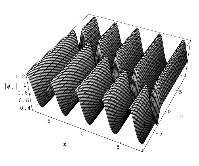
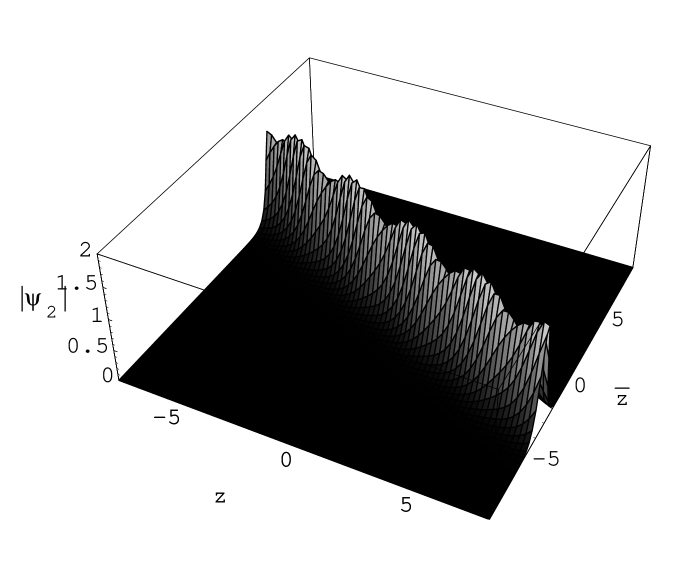
Figure 1: Dark-bright soliton pair of CNLS equation: $|\psi_{1}|$ shows a dark soliton residing on a cnoidal background. $|\psi_{2}|$ shows a bright soliton. The parameters are $v=0,k=0.9,p=1.3,u=-0.38+0.63i,M=1,N=0,C=0.3.$

The dark-bright pair soliton moves along a line which satisfies $|s_{2}|\sim|s_{0}^{(M)}|\sim|s_{1}^{(M)}|$ in Eq. (7). Here, $|s_{0}^{(M)}|$ or $|s_{1}^{(M)}|$ mean $M$-coupled terms in Eq. (7). Thus $|s_{0}^{(M)}|$ is obtained from $|s_{0}|$ in Eq. (7) by taking $M=1,N=0$. In the subsequent section, we use notations $|s_{0}^{(N)}|$ or $|s_{1}^{(N)}|$, which means $N$-coupled terms in Eq. (7). In this case, $|s_{0}^{(N)}|$ is obtained from $|s_{0}|$ in Eq. (7) by taking $M=0,N=1$. As we move away from the soliton, it becomes $|s_{2}|>>|s_{0}^{(M)}|\sim|s_{1}^{(M)}|$ or $|s_{2}|<<|s_{0}^{(M)}|\sim|s_{1}^{(M)}|$, and $\psi_{2}$ in Eq. (6) becomes zero. We can see from Eq. (7) that the dominating factor of $|s_{0}^{(M)}|$ (or $|s_{1}^{(M)}|$) is $\exp(-{\rm{Im}}\Delta)$. Other terms give much small oscillating behavior. The dominating factor of $|s_{2}|$ is $\exp({\rm{Im}}(\lambda^{2}\bar{z}-\lambda z)/2)$. Thus, the soliton pair moves along the line $z=\alpha\bar{z}$, where

$$\alpha={{\rm{Im}}(\lambda^{2}/2-\gamma+pv\beta)/{\rm{Im}}(\beta p+\lambda/2)}.$$ (10)

The value $\alpha$ of the soliton for parameters of Figure 1 is calculated to be -1.92 using Eq. (10), which is in accordance with Figure 1.

Another interesting feature of Figure 1 ($|\psi_{1}|$) is that the crest of the cnoidal background shifts constantly across the dark soliton. The shift is calculated as following. As we move away from the soliton such that $|s_{2}|>>|s_{0}^{(M)}|\sim|s_{1}^{(M)}|$, we find that $\psi_{1}^{c-s}(z,\bar{z})\rightarrow\psi_{1}^{c}(z,\bar{z})$ from Eq. (6). Thus $|\psi_{1}^{c-s}|\rightarrow p{\rm{dn}}\chi$ in this region. On the other side of the dark soliton, it becomes $|s_{2}|<<|s_{0}^{(M)}|\sim|s_{1}^{(M)}|$, and $\psi_{1}^{c-s}(z,\bar{z})\rightarrow\psi_{1}^{c}(z,\bar{z})+i(\lambda-\lambda^{*})(s_{1}^{(M)}/s_{0}^{(M)}+s_{0}^{(M)*}/s_{1}^{(M)*})^{-1}$. Using that $s_{1}^{(M)}/s_{0}^{(M)}=-e^{-i\zeta}{\rm{sn}}(-iu){\rm{dn}}(\chi+iu)/{\rm{cn}}(-iu)$ (Use Eqs. (7) and (25) with $N=0$), we find that (For simplicity, we take $u=iu_{I}$.)

$$\psi_{1}^{c-s}e^{-i\zeta}\rightarrow p~{}{\rm{dn}}\chi-2p{{\rm{dn}}u_{I}\over{\rm{cn}}u_{I}~{}{\rm{sn}}u_{I}}\left({{\rm{sn}}u_{I}{\rm{dn}}(\chi-u_{I})\over{\rm{cn}}u_{I}}+{{\rm{cn}}u_{I}\over{\rm{sn}}u_{I}{\rm{dn}}(\chi-u_{I})}\right)^{-1},$$ (11)

where we use Eqs. (9), (26) and ${\rm{sn}}u_{I}\equiv{\rm{sn}}(u_{I},k)$. Using the addition theorem, Eq. (11) can be written

$$p{{\rm{dn}}(\chi-u_{I}){\rm{dn}}u_{I}-k^{2}{\rm{sn}}u_{I}{\rm{cn}}u_{I}{\rm{sn}}(\chi-u_{I}){\rm{cn}}(\chi-u_{I})\over 1-k^{2}{\rm{sn}}^{2}u_{I}{\rm{sn}}^{2}(\chi-u_{I})}$$

$$-2p{{\rm{dn}}u_{I}{\rm{dn}}(\chi-u_{I})\over{\rm{sn}}^{2}u_{I}{\rm{dn}}^{2}(\chi-u_{I})+{\rm{cn}}^{2}u_{I}}$$

$$=p{-{\rm{dn}}(\chi-u_{I}){\rm{dn}}u_{I}-k^{2}{\rm{sn}}u_{I}{\rm{cn}}u_{I}{\rm{sn}}(\chi-u_{I}){\rm{cn}}(\chi-u_{I})\over 1-k^{2}{\rm{sn}}^{2}u_{I}{\rm{sn}}^{2}(\chi-u_{I})}$$

$$=-p{\rm{dn}}(\chi-2u_{I}).$$ (12)

Thus, $|\psi_{1}^{c-s}|\rightarrow p{\rm{dn}}(\chi-2u_{I})$ in this region, and the shift of crest is $2u_{I}$. For complex values of $u=u_{R}+iu_{I}$, we find the following identity which is checked numerically for various values of complex $u$ and real $\chi,k$.

$$|{\rm{dn}}(\chi,k)-\left({{\rm{dn}}(-iu,k)\over{\rm{cn}}(-iu,k){\rm{sn}}(-iu,k)}+{{\rm{dn}}(iu^{*},k)\over{\rm{cn}}(iu^{*},k){\rm{sn}}(iu^{*},k)}\right)\times$$

$$\left({{\rm{sn}}(-iu,k){\rm{dn}}(\chi+iu,k)\over{\rm{cn}}(-iu,k)}+{{\rm{cn}}(iu^{*},k)\over{\rm{sn}}(iu^{*},k){\rm{dn}}(\chi-iu^{*},k)}\right)^{-1}|={\rm{dn}}(\chi-2u_{I},k).$$ (13)

Using Eq. (13), we find that $|\psi_{1}^{c-s}|\rightarrow p{\rm{dn}}(\chi-2u_{I})=p{\rm{dn}}(\chi-2{\rm{Im}}u)$ still holds. We see that the parameter $u$ is suitable (compared to the DT parameter $\lambda$) in describing the characteristics of (soliton + cnoidal) system. The shift of the crest in terms of $z$ is $z\rightarrow z+{2{\rm{Im}}u/p}$ when we take $v=0$ in $\chi=-p(z-v\bar{z})$. In Figure 1, this shift is $0.97$.

3.2 Soliton on top of Cnoidal wave

Recently there arise new interests on optically-induced lattices and the localization of light in those gratings [16, 17, 18]. Especially, Ref. [18] describes a stationary configuration of (soliton + cnoidal wave) system where a soliton moves in parallel with the crest of a cnoidal wave. In this case, the velocity of the soliton is zero and Eq. (10) requires that $\lambda^{2}/2-\gamma+pv\beta$ should be a real number. It, in turn, requires that $u$ takes forms $u=iu_{I}$ or $u=iu_{I}+K^{\prime}$. To see this, use Eqs. (8), (9) and (26). Note that [31]

$${\rm{sn}}(a+iK^{\prime})={1\over{\rm{sn}}a},~{}{\rm{cn}}(a+iK^{\prime})=-{i\over k}{{\rm{dn}}a\over{\rm{sn}}a},~{}{\rm{dn}}(a+iK^{\prime})=-i{{\rm{cn}}a\over{\rm{sn}}a}.$$ (14)

Here $u_{I}$ is an real number and $K^{\prime}=K(\sqrt{1-k^{2}})$.

Fig. 2 shows one such case. Here solitons run in parallel with the crest of cnoidal wave. For this figure, we take $M=1.1,N=1$. In this case, there arises interference between the $M$ and $N$-coupled terms in $s_{0},s_{1}$ of Eq. (7). This interference results in an oscillating behavior of solitons as shown in Fig. 2.

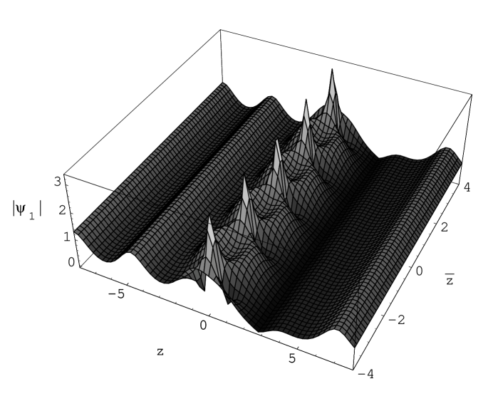
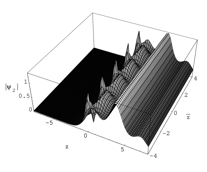
Figure 2: Dark-bright soliton pair moving paralelly along the crest of cnoidal wave: $|\psi_{1}|$ for dark soliton, $|\psi_{2}|$ for bright soliton. The parameters are $v=0,k=0.9,p=1.3,u=0.63i,M=1.1,N=1,C=0.3.$

The oscillating behavior disappears in the case of $N=0$ (or $M=0$), and we get a stationary configuration of (soliton + cnoidal wave) system. This case corresponds to the system discussed in [18]. (They use numerical analysis.) Various stationary configurations dealt in [18] can be obtained from our result in Eqs. (6) and (7) by taking proper values of parameters. It includes cases taking $k\geq 1$, $0\geq k\geq 1$, as well as taking $u=iu_{I}$ or $u=iu_{I}+K^{\prime}$ with $N=0$ (or $M=0$). More detailed characteristics of solutions corresponding to this specific choices of parameters are discussed elsewhere [32].

3.3 Soliton Fusion on a Cnoidal wave background

More general solution describing (soliton+cnoidal wave) is given by taking $M\neq 0,N\neq 0$ in Eq. (7). Figure 3 describes one of this case. We see that a dark-bright pair breaks up into another dark-bright pair plus an oscillating soliton.

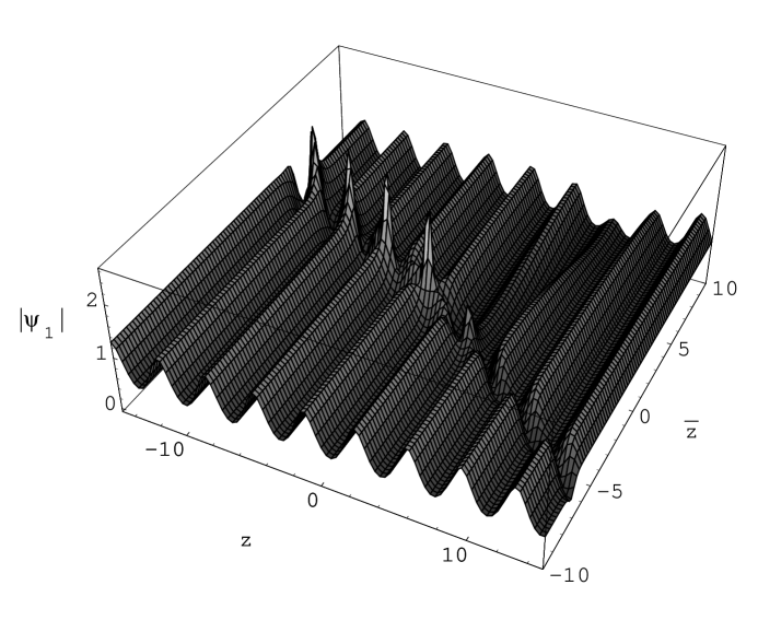
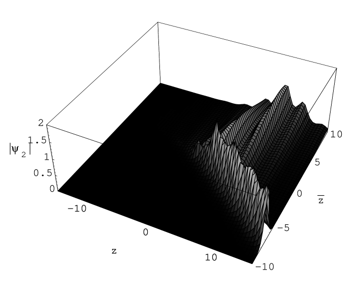
Figure 3: Dark-bright soliton pair breaks up into another dark-bright pair plus an oscillating soliton: $|\psi_{1}|$ shows a dark soliton breaking up into a dark plus oscillating solitons. $|\psi_{2}|$ shows a bright soliton changing its direction. The parameters are $v=0,k=0.9,p=1.3,u=-0.38+0.63i,M=1.1,N=1,C=0.3.$

This feature was first found in [5]. Our result is a generalization of the result in [5], such that a dark soliton resides on a cnoidal wave instead on a constant background.

There are three soliton lines in Fig. 3. The direction of these lines is calculated similarly as in the subsection 3.1. The directions of two dark-bright pairs are given by lines satisfying either $|s_{2}|\sim|s_{0}^{(M)}|\sim|s_{1}^{(M)}|$ or $|s_{2}|\sim|s_{0}^{(N)}|\sim|s_{1}^{(N)}|$. The direction of soliton line for $|s_{2}|\sim|s_{0}^{(M)}|\sim|s_{1}^{(M)}|$ is given in Eq. (10) of subsection 3.1. It was $z=-1.92\bar{z}$ for parameters of Fig. 1 (or Fig. 3). Contrary to the case of Fig. 1 (where the soliton exists on a full straight line), the soliton in Fig. 3 (which exists on a half of the line) exists only in the region satisfying $|s_{2}|\sim|s_{0}^{(M)}|\sim|s_{1}^{(M)}|>>|s_{0}^{(N)}|\sim|s_{1}^{(N)}|$. Using the expression for $\psi_{2}$ in Eq. (6), it is easy to see that the soliton disappears in the region $|s_{2}|\sim|s_{0}^{(M)}|\sim|s_{1}^{(M)}|<<|s_{0}^{(N)}|\sim|s_{1}^{(N)}|$.

Another dark-bright pair moves along a line satisfying $|s_{2}|\sim|s_{0}^{(N)}|\sim|s_{1}^{(N)}|$, or $z=\hat{\alpha}\bar{z}$, where

$$\hat{\alpha}={{\rm{Im}}(\lambda^{2}/2+\gamma-pv\beta)\over{\rm{Im}}(-\beta p+\lambda/2)}.$$ (15)

In this case, the dominating factor of $|s_{0}^{(N)}|$ (or $|s_{1}^{(N)}|$) in Eq. (7) is $\exp({\rm{Im}}\Delta)$. The dominating factor of $|s_{2}|$ is still $\exp({\rm{Im}}(\lambda^{2}\bar{z}-\lambda z)/2)$. Thus, the soliton pair moves along the line ${\rm{Im}}\Delta={\rm{Im}}(\lambda^{2}\bar{z}-\lambda z)/2)$, which gives Eq. (15). For parameters of Fig. 3, $\hat{\alpha}=0.44$.

The oscillating soliton in $|\psi_{1}|$ of Fig. 3 moves along a line $z=\tilde{\alpha}\bar{z}$, where

$$\tilde{\alpha}={{\rm{Im}}(-\gamma+pv\beta)\over{\rm{Im}}(\beta p)}.$$ (16)

In this case, the line is described by $|s_{0}^{(M)}|(\sim|s_{1}^{(M)}|)\sim|s_{0}^{(N)}|(\sim|s_{1}^{(N)}|)$. The dominating factor of $|s_{0}^{(M)}|$ (or $|s_{1}^{(M)}|$) is $\exp(-{\rm{Im}}\Delta)$, while that of $|s_{0}^{(N)}|$ (or $|s_{1}^{(N)}|$) is $\exp({\rm{Im}}\Delta)$. Thus, the oscillating soliton moves along a line ${\rm{Im}}\Delta=0$, which gives Eq. (16). For parameters of Fig. 3, $\tilde{\alpha}=-2.89$. Note that on a line of the oscillating soliton, it becomes $|s_{2}|<<|s_{0}|\sim|s_{1}|$. Thus there appears no soliton in $|\psi_{2}|$ along this line, see Eq. (6). The nature of the oscillating soliton in $\psi_{1}$ is exactly that of the single-component NLSE in [30]. In the region of $|s_{2}|>>|s_{0}|\sim|s_{1}|$, the oscillating soliton disappears even in $|\psi_{1}|$.

The shift of the crest of the cnoidal wave across the solitons can be similarly calculated as in the subsection 3.1. Especially in the region (Region I) where $|s_{2}|>>|s_{0}^{(M)}|\sim|s_{1}^{(M)}|$ and $|s_{2}|>>|s_{0}^{(N)}|\sim|s_{1}^{(N)}|$, we have $|\psi_{1}^{c-s}(z,\bar{z})|\rightarrow|\psi_{1}^{c}(z,\bar{z})|=p{\rm{dn}}(\chi)$. In the region (Region II) where $|s_{2}|<<|s_{0}^{(M)}|\sim|s_{1}^{(M)}|$ and $|s_{0}^{(N)}|\sim|s_{1}^{(N)}|<<|s_{0}^{(M)}|\sim|s_{1}^{(M)}|$, we have $\psi_{1}^{c-s}(z,\bar{z})\rightarrow\psi_{1}^{c}(z,\bar{z})+i(\lambda-\lambda^{*})(s_{1}^{(M)}/s_{0}^{(M)}+s_{0}^{(M)*}/s_{1}^{(M)*})^{-1}$ and $|\psi_{1}^{c-s}|\rightarrow p{\rm{dn}}(\chi-2u_{I})=p{\rm{dn}}(\chi-2{\rm{Im}}u)$, see subsection 3.1. In the region (Region III) where $|s_{2}|<<|s_{0}^{(N)}|\sim|s_{1}^{(N)}|$ and $|s_{0}^{(N)}|\sim|s_{1}^{(N)}|>>|s_{0}^{(M)}|\sim|s_{1}^{(M)}|$, we have $\psi_{1}^{c-s}(z,\bar{z})\rightarrow\psi_{1}^{c}(z,\bar{z})+i(\lambda-\lambda^{*})(s_{1}^{(N)}/s_{0}^{(N)}+s_{0}^{(N)*}/s_{1}^{(N)*})^{-1}$. In this case, $s_{1}^{(N)}/s_{0}^{(N)}=-e^{-i\zeta}{\rm{cn}}(-iu)/({\rm{dn}}(\chi-iu){\rm{sn}}(-iu))$. Similar procedure used in Eqs. (11) and (12) gives us $|\psi_{1}^{c-s}|\rightarrow p{\rm{dn}}(\chi+2u_{I})=p{\rm{dn}}(\chi+2{\rm{Im}}u)$.

Region I and Region II meat at a boundary, along which the dark-bright soliton pair moves with the velocity $\alpha$ in Eq. (10). Along the boundary between Region I and III, the soliton pair moves with the velocity $\hat{\alpha}$ in Eq. (15). Finally, the oscillating soliton moves along the boundary between Region II and III with the velocity $\tilde{\alpha}$ in Eq. (16). Thus the relative shift of the crest of the cnoidal wave across the boundary described by $\tilde{\alpha}$ is given by $\chi\rightarrow\chi-4{\rm{Im}}u$. Then the shift of the crest in terms of $z$ is $z\rightarrow z+{4{\rm{Im}}u/p}$ when we take $v=0$ in $\chi=-p(z-v\bar{z})$. For parameters of Figure 3, this shift is $1.94$.

4 Solution of defocusing medium

Figure 4 shows a dark soliton on a cnoidal background in a defocusing medium. It is obtained using Eqs. (5), (6), (7) and taking $\sigma=-1$, $v=0,k=0.9i,p=1.3i,u=-0.3-0.98i,M=1,N=0,C=0.1$. Note that in the case of defocusing medium ($\sigma=-1$), we take imaginary $k,p$. Another specific feature of the defocusing medium is that it is not permitted to take both $M$ and $N$ to be simultaneously nonzero. This fact is explained as following.

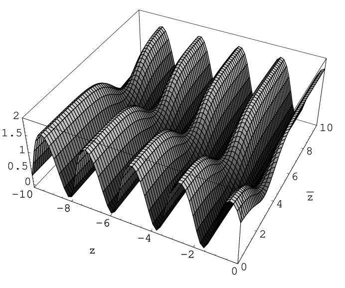
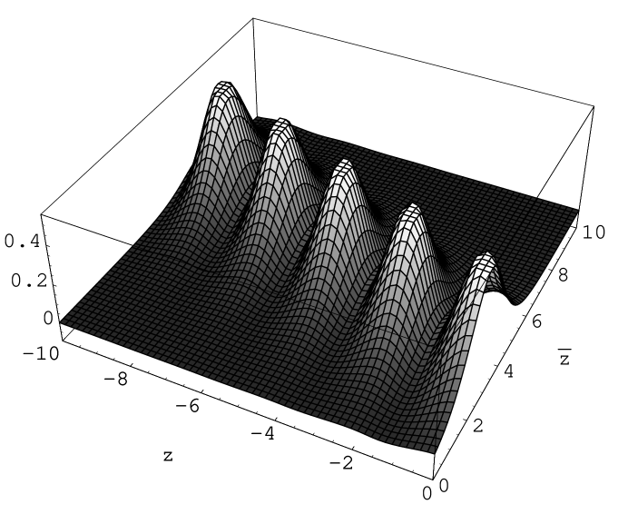
Figure 4: Dark-bright soliton pair moving in a defocusing medium: $|\psi_{1}|^{2}$, a dark soliton and $|\psi_{2}|^{2}$, a bright soliton. The parameters are $v=0,k=0.9i,p=1.3i,u=-0.3-0.98i,M=1,N=0,C=0.1$

The denominator part of Eq. (7) is $|s_{0}|^{2}-|s_{1}|^{2}-|s_{2}|^{2}$, which is required to be positive definite or negative definite on all $(z,\bar{z})$ plane. Otherwise, we will get an unphysical singular solution. But there always exists a region in the $(z,\bar{z})$ plane where $|s_{2}|>>|s_{0}|$, which means the denominator must be negative definite. Thus we need $|s_{0}|^{2}-|s_{1}|^{2}$ should be negative definite. In the region ${\rm{Im}}\Delta\sim-\infty$ where $|s_{0}|\sim|s_{0}^{(M)}|,|s_{1}|\sim|s_{1}^{(M)}|$, the negative definiteness requires $1<|s_{1}^{(M)}/s_{0}^{(M)}|=|{\rm{sn}}(-iu){\rm{dn}}(\chi+iu)/{\rm{cn}}(-iu)|$. On the other hand, in the region ${\rm{Im}}\Delta\sim\infty$ where $|s_{0}|\sim|s_{0}^{(N)}|,|s_{1}|\sim|s_{1}^{(N)}|$, we need $1<|s_{1}^{(N)}/s_{0}^{(N)}|=|{\rm{cn}}(-iu)/({\rm{dn}}(\chi-iu){\rm{sn}}(-iu))|$. As $|{\rm{dn}}(\chi\pm iu)|$ is an oscillating function of $\chi$, the negative definiteness from the two regions results in a contradiction on the magnitude of $|{\rm{sn}}(-iu)/{\rm{cn}}(-iu)|$. Thus we need one of $M,N$ should be zero. Thus there does not exist the phenomenon of soliton fusion in the case of defocusing medium.

When we take $N=0$ as in Fig. 4, we need $1<|{\rm{sn}}(-iu){\rm{dn}}(\chi+iu)/{\rm{cn}}(-iu))|$. In the appendix II, we prove that

$$(1+k^{2})^{(1/4)}\left|{{\rm{sn}}(-iu_{R}+m\tilde{K}^{\prime},ik)\over{\rm{cn}}(-iu_{R}+m\tilde{K}^{\prime},ik)}\right|=|{\rm{dn}}(\chi+iu_{R}-m\tilde{K}^{\prime},ik)|/(1+k^{2})^{(1/4)}=1,$$ (17)

where

$$\tilde{K}^{\prime}={K^{\prime}(1/\sqrt{1+k^{2}})\over 2\sqrt{1+k^{2}}},$$ (18)

$m$ is an odd number ($m=2n+1$), $\chi=-ip(z-v\bar{z})$ and $k,p,v,u_{R}$ are real numbers. (Here, we use the fact that $k\rightarrow ik,p\rightarrow ip$ in the defocusing medium.) We also found that

$$(1+k^{2})^{(1/4)}\left|{{\rm{sn}}(-iu_{R}+u_{I},ik)\over{\rm{cn}}(-iu_{R}+u_{I},ik)}\right|>1,~{}|{\rm{dn}}(\chi+iu_{R}-u_{I},ik)|/(1+k^{2})^{(1/4)}>1,$$ (19)

when

$$(4n+1)\tilde{K}^{\prime}<u_{I}<(4n+3)\tilde{K}^{\prime}$$ (20)

where $n$ is an arbitrary integer. On the outsides of interval in Eq. (20), Eq. (19) reverses its inequality sign. Thus we can see that the negative definiteness constrains the possible value of $u_{I}$ to the intervals given in Eq. (20). Similarly we must take the value $u_{I}$ in the outsides of intervals in Eq. (19) when we take $M=0$. For the parameters of Fig. 4, $\tilde{K}^{\prime}=0.67$.

The dark-bright pair soliton moves along a line, which satisfies $|s_{2}|\sim|s_{0}^{(M)}|\sim|s_{1}^{(M)}|$ ($N=0$ case). Thus we can use Eq. (10) to describe the direction of the soliton line. In the case of defocusing medium, we must take imaginary $p,k$ values. For parameters of Fig. 4, $\alpha=-2.48$. The soliton line shifts along the $\bar{z}$-axis (or $z$-axis) according to the relative magnitude of $M$ and $C$. This shift is rather large in Fig. 4 compared to the other figures, which is due to large $M/C=10$ value.

The shift of the crest for the case of defocusing medium is similarly calculated as in subsection 3.1. At the region $|s_{2}|>>|s_{0}^{(M)}|$, $\psi_{1}^{c-s}(-pi(z-v\bar{z}))=\psi_{1}^{c}(-pi(z-v\bar{z}))$. To calculate $\psi_{1}^{c-s}$ in the region the $|s_{2}|<<|s_{0}^{(M)}|$, we use the following formula

$$|{\rm{dn}}(i\chi,ik)-\left({{\rm{dn}}(-iu,ik)\over{\rm{cn}}(-iu,ik){\rm{sn}}(-iu,ik)}-{{\rm{dn}}(iu^{*},-ik)\over{\rm{cn}}(iu^{*},-ik){\rm{sn}}(iu^{*},-ik)}\right)\times$$

$$\left({{\rm{sn}}(-iu,ik){\rm{dn}}(i\chi+iu,ik)\over{\rm{cn}}(-iu,ik)}-{{\rm{cn}}(iu^{*},-ik)\over{\rm{sn}}(iu^{*},-ik){\rm{dn}}(-i\chi-iu^{*},-ik)}\right)^{-1}|$$

$$=|{\rm{dn}}(i\chi+2i{\rm{Re}}u,ik)|,$$ (21)

where $u$ is complex and $\chi,k$ are real. Then using Eqs. (6) and (21), we find that $|\psi_{1}^{c-s}(-pi(z-v\bar{z}))|=|\psi_{1}^{c}(-pi(z-v\bar{z})+2i{\rm{Re}}u)|$ for real $p$. The shift of the crest in terms of $z$ is $z\rightarrow z-{2{\rm{Re}}u/p}$ for the case of $v=0$. In Figure 4, this shift is $0.46$.

5 Conclusions

In this paper, we have introduced (soliton+cnoidal wave) solutions of the CNLS equation. They were obtained using the DT and introducing a solution of the associated linear problem on a cnoidal background. We calculate the moving direction of a soliton on a cnoidal background and the shift of the crest of a cnoidal wave. We also found a solution in the self-focusing case where a dark-bright pair breakup into another dark-bright pair and an oscillating soliton. These type of solutions, which can be easily applicable to the analysis of physically interesting processes, seem rather rare in the literature of physics. These solutions can be used, for example, in describing the localized states in optically induced refractive index gratings.

The stability analysis of these solutions is remained for future study. In fact, there already appears some numerical studies on this subject [18]. There was shown that the (soliton+ cnoidal wave) system is unstable or weakly stable for the focusing case, while it is stable for the defocusing case.

ACKNOWLEDGMENT

I am grateful to Yuri S. Kivshar for showing me the paper [18] prior to publication. This work was supported by Korea Research Foundation Grant (KRF-2003-070-C00011).

6 Appendix I: Proof of Sym’s solution

In this appendix, we show that $s_{0},s_{1},s_{2}$ in Eq. (7) indeed satisfy the linear equation (4). Consider the following equation, which is obtained from the $\partial_{z}$-part of Eq. (4);

$$\partial_{z}s_{0}+\psi_{1}^{c}s_{1}+i\lambda s_{0}/2=0.$$ (22)

By inserting $s_{0},s_{1}$ (For simplicity, we consider a case of $M=1,N=0$ in Eq. (7).) into Eq. (22) and taking $\psi_{1}^{c}$ as in Eq. (5), we get

$$-ip\beta-{p\over 2K}{\theta_{0}^{\prime}({\chi+iu\over 2K})\over\theta_{0}({\chi+iu\over 2K})}+{p\over 2K}{\theta_{0}^{\prime}({\chi\over 2K})\over\theta_{0}({\chi\over 2K})}-p~{}{\rm{dn}}(\chi,k){\theta_{1}({-iu\over 2K})\over\theta_{2}({-iu\over 2K})}{\theta_{3}({\chi+iu\over 2K})\over\theta_{0}({\chi+iu\over 2K})}+p{{\rm dn}(u,k^{\prime}){\rm cn}(u,k^{\prime})\over{\rm sn}(u,k^{\prime})}.$$ (23)

Inserting $\beta$ in Eq. (8) into Eq. (23) and using following identities [25, 31],

$$\int_{0}^{u}{\rm{dn}}^{2}u~{}du={1\over 2K}{\theta_{0}^{\prime}({u\over 2K})\over\theta_{0}({u\over 2K})}+{E\over K}u,$$ (24)

$${\rm sn}u={1\over\sqrt{k}}{\theta_{1}({u\over 2K})\over\theta_{0}({u\over 2K})},~{}{\rm cn}u={\sqrt{k^{\prime}}\over\sqrt{k}}{\theta_{2}({u\over 2K})\over\theta_{0}({u\over 2K})},~{}{\rm dn}u=\sqrt{k^{\prime}}~{}{\theta_{3}({u\over 2K})\over\theta_{0}({u\over 2K})},$$ (25)

$${\rm{sn}}(iu,k^{\prime})=i{{\rm{sn}}(u,k)\over{\rm{cn}}(u,k)},~{}{\rm{cn}}(iu,k^{\prime})={1\over{\rm{cn}}(u,k)},~{}{\rm{dn}}(iu,k^{\prime})={{\rm{dn}}(u,k)\over{\rm{cn}}(u,k)},$$ (26)

we get

$$-p\int^{\chi+iu}_{0}[{\rm{dn}}^{2}v-{\rm{dn}}^{2}(v-iu)]dv+{{\rm{sn}}(-iu,k)\over{\rm{cn}}(-iu,k)}[{\rm{dn}}(-iu,k)-{\rm{dn}}(\chi,k)~{}{\rm{dn}}(\chi+iu,k)].$$ (27)

Finally, using the following identity (It is a result of the addition theorem of Jacobi’s elliptic functions.)

$${\rm{dn}}^{2}(a-b)-{\rm{dn}}^{2}a=k^{2}{{\rm{sn}}b\over{\rm{cn}}b}[{\rm{cn}}a~{}{\rm{sn}}a~{}{\rm{dn}}(a-b)+{\rm{dn}}a~{}{\rm{cn}}(a-b)~{}{\rm{sn}}(a-b)]$$ (28)

$$= -{{\rm{sn}}b\over{\rm{cn}}b}{d\over da}[{\rm{dn}}a~{}{\rm{dn}}(a-b)],$$

we can see that Eq. (27) becomes zero. Other $\partial_{z}$-part of the linear equation (4) (including the $M=0,N=1$ case of $s_{0},s_{1}$ in Eq. (7)) are similarly proved.

A $\partial_{\bar{z}}$-part of Eq. (4) is ($\sigma=1$ case)

$$\partial_{\bar{z}}s_{0}+i|\psi_{1}^{c}|^{2}s_{0}-i\partial_{z}\psi_{1}^{c}~{}s_{1}-\lambda\psi_{1}^{c}s_{1}-i\lambda^{2}s_{0}/2=0.$$ (29)

By inserting $s_{0},s_{1}$ (For simplicity, we take $M=1,N=0$ in Eq. (7).) into the left part of Eq. (29) and taking $\psi_{1}^{c}$ as in Eq. (5), we get

$${i\over 2}[-p^{2}(2-k^{2})+{v^{2}\over 4}]-i\gamma-v({\partial_{z}s_{0}\over s_{0}}+i{v\over 4})+ip^{2}{\rm{dn}}^{2}\chi-{i\over 2}\lambda^{2}$$

$$+~{}p~{}[~{}i\partial_{z}{\rm{dn}}\chi+(\lambda+{v\over 2}){\rm{dn}}\chi]~{}{\theta_{1}({-iu\over 2K})\over\theta_{2}({-iu\over 2K})}{\theta_{3}({\chi+iu\over 2K})\over\theta_{0}({\chi+iu\over 2K})}.$$ (30)

Using Eq. (22) and the identity (25), Eq. (30) becomes

$$-{i\over 2}p^{2}(2-k^{2})+{i\over 8}v^{2}+i{p^{2}\over 2}[{\rm{dn}}^{2}(u,k^{\prime})+{{\rm{cn}}^{2}(u,k^{\prime})\over{\rm{sn}}^{2}(u,k^{\prime})}]+{i\over 2}\lambda v-{i\over 4}v^{2}-{i\over 2}\lambda^{2}$$

$$+ip^{2}{\rm{dn}}^{2}\chi-({p\over 2}v{\rm{dn}}\chi-ip^{2}k^{2}{\rm{sn}}\chi{\rm{cn}}\chi-\lambda p{\rm{dn}}\chi){{\rm{sn}}(-iu,k)\over{\rm{cn}}(-iu,k)}{\rm{dn}}(\chi+iu,k).$$ (31)

With the help of Eqs. (26) and (9), repeated applications of addition theorem on Eq. (31) gives zero, which proves Eq. (29). Other $\partial_{\bar{z}}$-part of the linear equation (4) (including the $M=0,N=1$ case of $s_{0},s_{1}$ in Eq. (7)) are similarly proved.

7 Appendix II: Proof of Eq. (17)

We first start with

$$(1+k^{2})^{(1/4)}{{\rm{sn}}(-iu,ik)\over{\rm{cn}}(-iu,ik)}=i{\rm{sn}}(-\sqrt{1+k^{2}}u,\tilde{k})/(1+k^{2})^{(1/4)},$$ (32)

where $\tilde{k}={1/\sqrt{1+k^{2}}}$ with $k$ real and $u$ is a complex value. By inserting $u=u_{R}+i\tilde{K}^{\prime}$ in Eq. (18) and using the addition theorem, Eq. (32) becomes

$${{\rm{sn}}(-\sqrt{1+k^{2}}u_{R},\tilde{k})(1+\tilde{k})-i{\rm{cn}}(-\sqrt{1+k^{2}}u_{R},\tilde{k}){\rm{dn}}(-\sqrt{1+k^{2}}u_{R},\tilde{k})\over 1+\tilde{k}{\rm{sn}}(-\sqrt{1+k^{2}}u_{R},\tilde{k})},$$ (33)

where we use

$${\rm{sn}}(-i\sqrt{1+k^{2}}\tilde{K}^{\prime},\tilde{k})=-i(1+k^{2})^{(1/4)},~{}{\rm{dn}}(-i\sqrt{1+k^{2}}\tilde{K}^{\prime},\tilde{k})=\sqrt{1+\tilde{k}},$$

$${\rm{cn}}(-i\sqrt{1+k^{2}}\tilde{K}^{\prime},\tilde{k})=(1+k^{2})^{(1/4)}\sqrt{1+\tilde{k}}.$$ (34)

It is now easy to see that the absolute value of Eq. (33) is 1.

In the case of ${\rm{dn}}$ formula,

$${\rm{dn}}(-iu,ik)/(1+k^{2})^{(1/4)}={{\rm{cn}}(-\sqrt{1+k^{2}}u,\tilde{k})\over{\rm{dn}}(-\sqrt{1+k^{2}}u,\tilde{k})(1+k^{2})^{(1/4)}}.$$ (35)

Applying a similar procedure used in obtaining Eq. (33) to Eq. (35) gives

$${{\rm{cn}}(-\sqrt{1+k^{2}}u_{R},\tilde{k})+i{\rm{sn}}(-\sqrt{1+k^{2}}u_{R},\tilde{k}){\rm{dn}}(-\sqrt{1+k^{2}}u_{R},\tilde{k})\over{\rm{dn}}(-\sqrt{1+k^{2}}u_{R},\tilde{k})-i\tilde{k}{\rm{cn}}(-\sqrt{1+k^{2}}u_{R},\tilde{k}){\rm{sn}}(-\sqrt{1+k^{2}}u_{R},\tilde{k})},$$ (36)

whose absolute value is 1. It is easy to expand above results to the case of $u=u_{R}-i\tilde{K}^{\prime}$. Using that ${\rm{sn}}(-iu,ik)/{\rm{cn}}(-iu,ik),{\rm{dn}}(-iu,ik)$ are periodic functions in $u_{I}$ with the period $2\tilde{K}^{\prime}$, we can obtain the result in Eq. (17) in subsection 4.

To obtain a result shown in Eq. (19), we should go through similar procedures in the above paragraphs with much complex expressions in this case. Instead of going through a tedious calculation, we use MAPLE to check numerically the validity of Eq. (19).

References

- [1] Manakov S V 1973 Zh. Eksp. Teor. Fiz. 65 505; 1974 Sov. Phys. JETP 38 248
- [2] Agrawal G P 1995 Nonlinear Fiber Optics ( New York: Academic )
- [3] Zakharov V E and Shabat A B 1974 Funct. Anal. Appl. 8 43
- [4] Berkhoer A L and Zakharov V E 1970 Zh. Eksp. Teor. Fiz. 58 903; 1970 Sov. Phys. JETP 31 486
- [5] Park Q H and Shin H J 2000 Phys. Rev. E 61 3093
- [6] Kivshar Y S and Luther-Davies 1998 Phys. Rep. B 298 81
- [7] Hioe F T 1999 Phys. Rev. Lett. 82 1152; 1998 Phys. Rev. E 58 6700
- [8] Florjanczyk M and Tremblay R 1989 Phys. Lett. A 141 34
- [9] Romeiras F J and Rowlands G 1986 Phys. Rev. A 33 3499
- [10] Shin H J 2003 J. Phys. A 36, 4113
- [11] Adams M R, Harnad J and Hurtubisc J 1993 Commun. Math. Phys. 155 385
- [12] Alfinito E, Leo M, Soliani G and Solombrino L 1995 Phys. Rev. E 53 3159
- [13] Polymilis C, Hizanidis K and Frantzeskakis D J 1998 Phys. Rev. E 58 1112
- [14] Porubov A V and Parker D F 1999 Wave Motion 29 97
- [15] Pulov V I, Uzunov I M and Chakarov E J 1998 Phys. Rev. E 57 3468
- [16] Efremidis N K, Sears S, Christodoulides D N, Fleisher J W, and Segev M 2002 Phys. Rev. E 66 046602
- [17] Fleischer J W, Segev M, Efremidis N K, and Christodoulides D N 2003 Phys. Rev. Lett. 90 023902; 2003 Nature 422 147; Neshev D, Ostrovskaya E, Kivshar Y and Krolikowski W 2003 Opt. Lett. 28 710
- [18] Desyatnikov A S, Ostrovskaya E A, Kivshar Y S and Denz C 2003 Phys. Rev. Lett. 91 153902-4
- [19] Lederer F, Darmanyan S, and Kobyakov A 2001 in Spatial Solitons (eds Trillo S, Torruellas W) 269 (Springer, New York).
- [20] Manakov S V 1973 Zh. Eksp. Teor. Fiz. 65 505 [1974 Sov. Phys. JETP 38 248]
- [21] Radhakrishnan R and Lakshmanan M 1995 J. Phys. A 28 2683
- [22] Sheppard A P and Kivshar Y S 1997 Phys. Rev. E 55 4773
- [23] Abdullaev F, Darmanyan S and Khabibullaev P 1993 Optical Solitons , Springer series in Nonlinear Dynamics (Springer-Verlag, Heidelberg)
- [24] see, for example, Kamchatnov A 1997 Phys. Rep. 286 199
- [25] Encyclopedic Dictionary of Mathematics by the Mathematical Society of Japan 1993 edited by K. Itô (The MIT press, Cambridge, Massachusetts)
- [26] Matveev V and Salle M 1990 Darboux Transformations and Solitons, Springer series in Nonlinear Dynamics (Springer-Verlag, Heidelberg)
- [27] Park Q Hand Shin H J 2001 Physica D 157 1
- [28] Park Q H and Shin H J 2002 IEEE J. Select. Topics Quantum Electron. 8 432
- [29] Sym A 1988 Fluid Dynamics research 3 151
- [30] Shin H J 2001 Phys. Rev. E 63 026606
- [31] Table of integrals, series, and products 1980 edited by Gradshteyn I S and Ryzhik I M(Academic press, New York)
- [32] Shin H J, to be published.