Synchronization and oscillator death in oscillatory media with stirring

Abstract

The effect of stirring in an inhomogeneous oscillatory medium is investigated. We show that the stirring rate can control the macroscopic behavior of the system producing collective oscillations (synchronization) or complete quenching of the oscillations (oscillator death). We interpret the homogenization rate due to mixing as a measure of global coupling and compare the phase diagrams of stirred oscillatory media and of populations of globally coupled oscillators.

The problem of synchronization of a large population of non–linear oscillators has received a great deal of attention lately sync due to its applications in a variety of physical josephson , chemical chem and biological systems winfree ; yeast , social phenomena clapp etc. Typically two types of couplings are used to describe the interactions in such systems: i.) global coupling, where each of the oscillators is coupled to all the others, or ii.) local coupling, where only the nearest neighbors are interacting. Global coupling is relevant for oscillators communicating via visual or acoustic signals, like flashing fireflies, chirping crickets, clapping audiences, and can also be implemented by electric coupling (see chem for a recent experiment on synchronization of globally coupled electrochemical oscillators). In these cases the time necessary for information to spread over the whole system is much shorter than the period of the oscillations. In general, global coupling leads to synchronization when the coupling is sufficiently strong and the distribution of the natural frequencies is not too broad.

In a continuous oscillatory medium (e.g. reaction-diffusion system) the oscillations at different points of the medium interact through molecular diffusion. Since the time-scale of diffusive transport on macroscopic lengthscales ($L$) is typically much longer than the characteristic timescale of the oscillations, $L^{2}/D\gg T_{osc}$, diffusion is unable to produce synchronized oscillations over the whole domain and the only coherent behavior appears in form of propagating waves wave1 ; wave2 .

In certain situations the oscillators are embedded into a moving medium, e.g. in a fluid flow. Examples are oscillatory chemical or biological systems in stirred reactors (Belousov-Zhabotinsky reaction wave2 , metabolic oscillations in cell suspensions yeast ), or in geophysical context: oceanic plankton populations plankton and chemical reactions in the atmosphere atmos transported by large scale geophysical flows. However, the effect of stirring in oscillatory media has not yet been investigated. It is often assumed, that strong stirring leads to spatially uniform concentrations, and thus the temporal evolution, simply described by a set of ordinary differential equations, becomes independent of the stirring process. But in most real systems there are inherent inhomogeneities imposed by boundary conditions or non-uniformities of certain external parameters. This can be due to spatial variations of temperature or illumination in a chemical reactor, or non-uniform distribution of sources in environmental flows. Therefore perfectly uniform concentrations are unattainable and stirring effects cannot be ignored.

In this Letter we investigate the behavior of a stirred oscillatory medium, described by a set of reaction-advection-diffusion equations

$${\partial_{t}C_{i}}+{\bf v}({\bf r},t)\nabla C_{i}=F_{i}(C_{1},...,C_{N};{\bf r})+D\Delta C_{i},$$ (1)

where $C_{i}({\bf r},t),i=1,2,...,N$, are the concentrations of $N$ interacting species advected by an incompressible fluid flow ${\bf v}({\bf r},t)$. The velocity field is assumed to be time-dependent, that ensures efficient mixing by the chaotic motion of the fluid elements mixing . The functions $F_{i}$ describe the nonlinear interactions between the components (chemical reactions, evolution of biological populations etc.) such that the local dynamics has a stable limit cycle in each point of the medium

$$\dot{C}_{i}=F_{i}(C_{1},...,C_{N};{\bf r})\to C_{i}(t+T_{\bf r};{\bf r})=C_{i}(t;{\bf r}).$$ (2)

The explicit dependence of the interaction terms on the spatial coordinate accounts for inhomogeneities of the medium. We consider the simplest form of inhomogeneity, when the medium is composed by identical oscillators except for their frequencies, that is non-uniform in space

$$F_{i}(C_{1},...,C_{N};{\bf r})=(1+\delta f({\bf r}))F^{\prime}_{i}(C_{1},...,C_{N}),$$ (3)

where $f({\bf r})$ and $\delta$ describe the shape and the amplitude of the inhomogeneity. We assume, for simplicity, that $\langle f({\bf r})\rangle=0$ and $\langle f^{2}({\bf r})\rangle=1$, where $\langle\;\;\rangle$ represents averaging over the domain.

Figure 1: Time-dependence of the mean concentration $\langle C_{1}\rangle$ for different stirring rates ($\nu$) and $\delta=0.2$.

In the numerical simulations stirring is modelled by a sinusoidal shear flow with alternating directions

$$v_{x}=(A/T)\sin(2\pi y+\phi_{n}),v_{y}=0$$

$$\;\;\;\;\;\;\;{\rm for}\;\;\;\;t\in[nT,(n+1/2)T)$$

$$v_{x}=0,v_{y}=(A/T)\sin(2\pi x+\phi_{n})$$

$$\;\;\;\;\;\;\;{\rm for}\;\;\;\;t\in[(n+1/2)T,(n+1)T)$$ (4)

($A=1.4$) advecting chaotically all fluid particles within the unit square with doubly periodic boundary conditions. The phases $\phi_{n}$ are chosen at random in each half period. This ensures that there are no transport barriers and all fluid elements can approach any other fluid element in the domain. We note that chaotic advection is a generic feature of simple time-dependent flows, therefore the results are expected to be characteristic to a broad range of fluid flows. We define the stirring rate as $\nu\equiv 1/T$, that is controlled by the period of the flow.

For the oscillatory dynamics the well known Lengyel-Epstein model of the chlorine–iodine–malonic acid reaction (CDIMA) wave2 is considered

$$F^{\prime}_{1}(C_{1},C_{2})=1-C_{1}-{4C_{1}C_{2}}/({b+C_{1}^{2}})$$

$$F^{\prime}_{2}(C_{1},C_{2})=a(C_{1}-{C_{1}C_{2}}/({b+C_{1}^{2}})).$$ (5)

The chemical dynamics has a uniform steady state, ($C_{1}^{*}=0.2,C_{2}^{*}=b+0.04$) which is unstable for the parameter values used, $b=0.005$, $a=0.375$, and the only attractor is a limit cycle. The shape of the inhomogeneity is chosen to be $f(x,y)=\sqrt{2}\sin(2\pi(x-y))$. The system (3-5) is investigated for different stirring rates $\nu$ and degrees of inhomogeneity $\delta$. ($D=10^{-4}$ in all simulations.)

Let us first discuss some special cases. For non-reactive components ($F(C_{1},..,C_{N})\equiv 0$) an initially non-uniform concentration is homogenized by mixing. In flows with chaotic advection the decay of the spatial fluctuations is exponential in time eigenmode

$$\langle(C-\langle C\rangle)^{2}\rangle\sim\exp(-2\alpha t),$$ (6)

and for long times the spatial structure is dominated by the eigenmode of the advection-diffusion operator ${\cal L}_{mix}\equiv D\Delta-{\bf v}\cdot\nabla$ with the largest (least negative) eigenvalue.

$$C({\bf r},t)\to\langle C({\bf r},0)\rangle+e^{-\alpha t}\Phi_{1},\;\;\;\;{\cal L}_{mix}\Phi_{i}=-\alpha_{i}\Phi_{i}.$$ (7)

Strictly speaking the eigenmodes have a temporal dependence following the evolution of the velocity field, but they are stationary at least in a statistical sense.

In a uniform oscillatory medium, $\delta=0$, the advection-reaction-diffusion problem has a spatially uniform oscillatory solution. This is stable to spatially non-uniform perturbations, and numerical simulations suggest that it is globally attracting. The decay of the spatial fluctuations is controlled by the chaotic mixing, as indicated by the exponential decay of the variance with the same exponent as for the non-reactive case. The only difference is that there are oscillations superposed due to the oscillatory nature of the chemical dynamics, i.e. $\langle(C-\langle C\rangle)^{2}\rangle\sim h(t)\exp(-2\alpha t)$ where $h(t)$ is periodic with the period of the oscillations of the mean field.

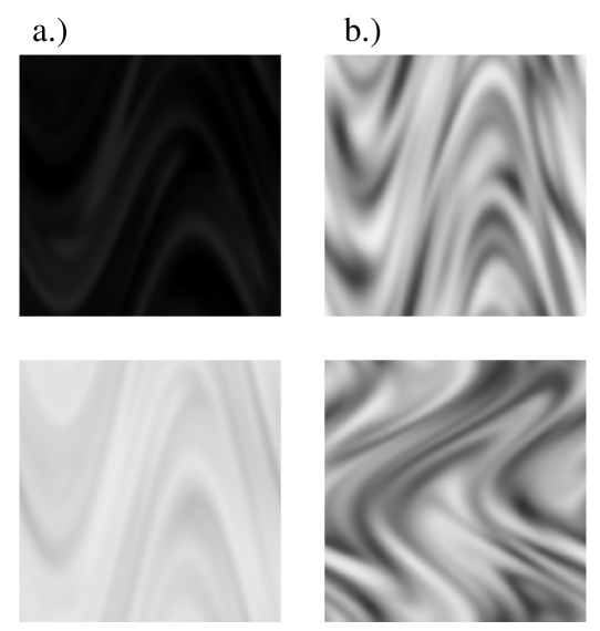
Figure 2: Snapshots of the concentration field $C_{1}(x,y)$ in the synchronized ($a.)\nu=0.4$) and the non-synchronized ($b.)\nu=0.167$) regimes ($\delta=0.2$)

Let us now consider a fixed amplitude of the inhomogeneity and vary the stirring rate. When stirring is strong the mean concentration has an oscillatory time-dependence indicating synchronization (Fig.1), but unlike in the case of the homogeneous medium, the spatial fluctuations do not disappear completely, since there is no spatially uniform oscillatory solution for $\delta>0$. For very fast stirring the spatial fluctuations are weak and the oscillations of the mean concentrations are almost the same as for a uniform medium. The amplitude of the oscillations of the mean field decreases with the stirring rate, while the frequency remains the same. On longer time scales, there is also a weak irregular modulation of the amplitude, that becomes more pronounced for slow stirring. When the stirring rate falls below a certain critical value, the synchronized oscillations disappear, and the mean concentration is almost constant apart from small irregular fluctuations.

Figure 3: Projection of the concentration field $C_{1}(x,y)$ on the chemical phase plane $C_{1}-C_{2}$ in the synchronized (a.) and non-synchronized case, $\delta=0.2$. The limit cycle for a single oscillator is also shown for reference.

Two pairs of snapshots of the concentration field $C_{1}(x,y)$, for the synchronized (a.) and unsynchronized (b.) case, are shown in Fig.2. The complex spatial structure, characteristic to chaotic mixing, is combined with a coherent time-evolution for supercritical stirring, while in the slow stirring case the snapshots corresponding to different times are statistically equivalent. The difference between the two regimes is also clearly visible on the projections of the concentration field onto the chemical phaseplane $C_{1}-C_{2}$ (Fig.3). When the stirring is strong the projected concentration fields appear as a small clump moving around the limit cycle of a single oscillator, while in the unsynchronized regime they extend over a large domain, that remains almost unchanged in time.

To characterize the degree of synchronization we calculate the standard deviation in time of the spatially averaged concentrations

$$R\equiv\sqrt{\frac{1}{\tau}\int_{t}^{t+\tau}\langle C\rangle^{2}dt^{\prime}-\left(\frac{1}{\tau}\int_{t}^{t+\tau}\langle C\rangle dt^{\prime}\right)^{2}},$$ (8)

for different stirring rates (Fig.4). Large values of $R$ indicate synchronization. $R(\nu,\delta)$ can be normalized by dividing it with the same quantity obtained for the uniform oscillating medium, $R_{0}=R(\delta=0)$ ($0<R/R_{0}<1$). The order parameter $R/R_{0}$ increases sharply above a critical stirring rate. In the unsynchronized regime, below the critical stirring rate, the order parameter is small. We believe, that in this regime $R$ tends to zero in the $D\to 0$ limit, that is analogous to the limit of infinitely many oscillators in the case of global coupling.

Figure 4: The normalized order parameter as a function of stirring rate for different degrees of non-uniformity of the medium.

The critical stirring rate depends on $\delta$, faster stirring is needed for synchronization when the medium has a larger spread of the local frequencies. When $\delta$ is sufficiently large a new regime appears between the synchronized and unsynchronized states. At intermediate stirring rates the oscillations of the mean field disappear completely (R=0) and the concentrations become uniform in space. This ’oscillator death’ state corresponds to the unstable equilibrium of the homogeneous chemical system, $C_{i}^{*}$. Thus, stirring in the presence of inhomogeneity can stabilize the unstable steady state of the chemical dynamics and suppress the oscillations. This results from the competition between the inhomogeneity of the medium generating non-uniform concentrations and mixing that tends to reduce the spatial fluctuations.

Similar regimes have been observed in ensembles of globally coupled oscillators Ermentrout ; PRL . In the stirred media due to the relative displacement of different parts of the medium the neighborhood of each point is changing in time, thus regions that are initially far from each other can interact at a later time. This defines a characteristic timescale of mixing as the time needed to bring pairs of points, initially separated by a distance comparable with the size of the domain, sufficiently close so that they can interact by diffusion. When this time is much shorter than the period of the oscillations, there is an effective global interaction in the moving medium. Thus the character and strength of the coupling can be controlled by the stirring rate. An analogous situation occurs in an ensemble of oscillators coupled through a network in which each node has a small number of connections that are changing in time in a random fashion network .

Figure 5: Phase diagram of the oscillatory medium with stirring (a.) and global coupling (b.) - the symbols represent: synchronization ($\blacksquare$), oscillator death ($\ast$) and no synchronization ($\odot$). The dashed line is the phase boundary based on equation (10).

The dynamics of globally coupled oscillators in the continuum limit is described by

$$\partial_{t}C_{i}=(1+\delta f({\bf r}))F_{i}(C_{1},..,C_{N})+\alpha_{g}(\langle C_{i}\rangle-C_{i}).$$ (9)

Similarly to the mixed system, in the absence of oscillations ($F_{i}(C_{1},..,C_{N})\equiv 0$), global coupling leads to an exponential decay of the concentration fluctuations, ${\rm Var}(C)\sim\exp(-2\alpha_{g}t)$. Based on this analogy, we interpret the homogenization rate in the stirred system, $\alpha$, as a measure of the coupling strength resulting from the combined effects of advection and diffusion.

In Fig.5 we present phase diagrams, both for the case of mixing and global coupling. The homogenization rate, $\alpha$, corresponding to different stirring rates have been obtained numerically by measuring the decay rate of the variance of the concentration field for a non-reactive component. In the fast stirring limit ($\nu L^{2}/D\gg 1$) the homogenization rate tends to be proportional with the stirring rate. The two phase diagrams have a qualitatively similar structure. Both strong coupling and fast stirring leads to synchronization, or oscillator death when the inhomogeneity of the medium is strong. Slow stirring is analogous to weak coupling as shown by the lack of synchronization in this regime.

For globally coupled oscillators an approximation for the boundary between the synchronization and oscillator death phase has been found recently in PRL

$$\alpha_{c}(\delta)=\lambda\left[\left({\omega}/{\lambda}\right)^{2}-1\right]\delta^{2},$$ (10)

where $\lambda$ and $\omega$ are the real and complex parts of the eigenvalue of the unstable steady state $C^{*}$. The above result is valid when $\omega\gg\lambda$, in our case $\lambda=0.222$ and $\omega=2.878$. We find that in the case of global coupling the boundary (10) agrees well with the numerical results. For the mixed system, however, the same boundary is shifted toward lower stirring rates/stronger inhomogeneity.

This is not surprising since the advection-diffusion operator has a complex structure and is not simply equivalent to a linear relaxation to the mean concentration. Although the long time decay of the fluctuations is dominated by the eigenmode with the largest eigenvalue, $\alpha=\alpha_{1}$, by replacing mixing with global coupling corresponding to the most slowly decaying eigenmode we underestimate the strength of the coupling due to mixing. This may be the explanation for the difference between the two diagrams in Fig.5. Another origin of the deviation could be that in the system with mixing fluid parcels move during a period of the flow and therefore the average value of the shape function $f(x,y)$ calculated along fluid trajectories has a smaller variance than in a motionless medium, resulting in a weaker effective inhomogeneity of the medium.

In summary, we have shown that oscillatory media with stirring exhibit qualitatively similar behavior to populations of globally coupled oscillators, and the effective coupling strength is controlled by the stirring rate. Changes in the stirring rate can lead to transitions to synchronization or oscillator death. This may explain some of the stirring effects observed in laboratory experiments Noszticzius and could also be exploited for controlling the dynamics of oscillatory systems. Similar behavior may also arise in systems where the local dynamics is chaotic.

We thank Silvia De Monte, Peter H. Haynes and Francesco d’Ovidio for useful discussions.

References

- (1) A. Pikovsky, M. Rosenblum, J. Kurths; Synchronization: A universal concept in nonlinear science, Cambridge University Press, 2001; S.H. Strogatz, Physica D 143, 1 (2000)
- (2) K. Wiesenfeld, P. Colet, S.H. Strogatz, Phys. Rev. Lett. 76, 404 (1996)
- (3) I.Z. Kiss, Y. Zhai, J.L. Hudson, Science, 296, 1676 (2002).
- (4) A.T. Winfree, The geometry of biological time, Springer, 2000.
- (5) S. Dano, P.G. Sorensen, F. Hyne, Nature 402, 320 (1999).
- (6) Z. Néda et al, Nature 403, 849 (2000).
- (7) Y. Kuramoto, Chemical oscillations waves and turbulence, Springer-Verlag, 1984
- (8) I.R. Epstein, K. Showalter, J. Phys. Chem. 100, 13132 (1996)
- (9) J. Huisman, F. J. Weissing, Nature 402, 407 (1999)
- (10) D. Poppe, H. Lustfeld, J. Geophys. Res. 101 D9, 14373 (1996)
- (11) H. Aref, J. Fluid Mech. (1984); Phys. Fluids 14, 1315 (2002)
- (12) R. Pierrehumbert, Chaos, Solitons Fractals 4, 1091 (1994), D. Fereday et al, Phys. Rev. E 65, 035301(R) (2002), J. Sukhatme, R.T. Pierrehumbert, Phys. Rev. E. 66, 056302 (2002)
- (13) G.B. Ermentrout, Physica D 41, 219 (1990); R.E. Mirollo, S.H. Strogatz, J. Stat. Phys. 60, 245 (1990);
- (14) S. De Monte, F. d’Ovidio, E. Mosekilde, Phys. Rev. Lett. 90, 054102 (2003).
- (15) V.N. Belykh (private communication).
- (16) Z. Noszticzius et al., J. Phys. Chem. 95, 6575 (1991)