Lyapunov Spreading of Semi-classical Wave Packets for the Lorentz Gas:
Theory and Applications

Abstract

We consider the quantum mechanical propagator for a particle moving in a $d$-dimensional Lorentz gas, with fixed, hard sphere scatterers. To evaluate this propagator in the semi-classical region, and for times less than the Ehrenfest time, we express its effect on an initial Gaussian wave packet in terms of quantities analogous to those used to describe the exponential separation of trajectories in the classical version of this system. This result relates the spread of the wave packet to the rate of separation of classical trajectories, characterized by positive Lyapunov exponents. We consider applications of these results, first to illustrate the behavior of the wave-packet auto-correlation functions for wave packets on periodic orbits. The auto-correlation function can be related to the fidelity, or Loschmidt echo, for the special case that the perturbation is a small change in the mass of the particle. An exact expression for the fidelity, appropriate for this perturbation, leads to an analytical result valid over very long time intervals, inversely proportional to the size of the mass perturbation. For such perturbations, we then calculate the long-time echo for semi-classical wave packets on periodic orbits. This paper also corrects an earlier calculation for a quantum echo, included in a previous paper, (nlin.CD/0307025). We explain the reasons for this correction.

I Introduction

The search for signatures of classical chaos in corresponding quantum systems is one of the main themes of quantum chaos. The literature in this subject is large, much of it described in recent books by Haake and by Stöckmann haake ; stock . Here we consider a simple version of this question, namely, we describe a semi-classical calculation of the short time spreading of a wave-packet for the quantum version of a classically chaotic system and show, as one might expect, that it is governed to a large extent by the Lyapunov exponents characterizing the exponential separation of close trajectories of the classical system. We consider a Lorentz gas, which consists of a particle, or a collection of non-interacting particles, moving in $d$-dimensions among a collection of fixed scatterers, generally taken to be $d$-dimensional hard spheres, with finite horizon. The case where the scatterers are centered at the vertices of a regular lattice is the Sinai billiard. Related work on this problem has been done by Wirzba wirz , which will be mentioned in Section II.

We consider the propagator for a semi-classical particle moving among the scatterers. The de Broglie wave length of the moving particle is taken to be small compared both to the size of a scatterer and to the average distance between scatterers. The propagator is evaluated by semi-classical methods for time intervals where a number of collisions take place. As long as the wave-packet remains small, its spreading with time is governed by a set of equations that are the quantum counterparts to the curvature equations of Sinai and co-workers sinai that determine the Lyapunov exponents and Kolmogorov-Sinai (KS) entropy for the classical system. We can then easily relate the spreading of the wave-packet to the classical Lyapunov exponents.

Next we apply this result to a calculation of the wave-packet auto-correlation function (the return probability), $C(t)$, defined by

$$C(t)=\left|\langle 0|e^{-itH/\hbar}|0\rangle\right|^{2},$$ (1)

where $H$ is the Hamiltonian of the system and $|0\rangle$ is an initial quantum state. We find that, for wave packets on periodic orbits, this function exhibits a series of maxima, with amplitudes decreasing mainly exponentially with time, as $\exp(-h_{\mathrm{KS}}t)$, where $h_{\mathrm{KS}}=\sum_{i}\lambda_{i}$ is the classical KS-entropy, and the $\lambda_{i}$ are the positive Lyapunov exponents for the corresponding periodic orbits. This type of decay of the auto-correlation function was first described by Heller heller . Here we also calculate the coefficient in front of the exponential. This coefficient has a sub-exponential time dependence. The auto-correlation function exhibits a set of maxima separated by deep minima that appear for simple physical reasons, as we explain in Section III.

These results are limited in applicability to times less than the Ehrenfest time, which is the time necessary for a wave packet to spread to the size of a scatterer. However, there is an application of them to the Loschmidt echo, or quantum fidelity, of a special type which is valid for a much larger time interval, greater than the Ehrenfest time. The Loschmidt echo peres ; past ; cucc , $M(t)$, is defined by

$$M(t)=\left|\langle 0|e^{it(H+\Sigma)/\hbar}e^{-itH/\hbar}|0\rangle\right|^{2}.$$ (2)

Here $H$ is the Hamiltonian for the system, $\Sigma$ is a small perturbing Hamiltonian, and $|0\rangle$ is some initial quantum state. For the case that $H$ is the Lorentz gas Hamiltonian with hard sphere scatterers, and the perturbation is a small change in the mass of the moving particle, it is straightforward to show that $M(t)$ is equal to the wave-packet autocorrelation function evaluated at a scaled time, which can be made to be much shorter than the physical time $t$, by choosing a suitably small mass perturbation. Therefore for this special perturbation and hard sphere Lorentz gas system, the quantum fidelity can be evaluated for very long times, if one knows the behavior of the auto-correlation function for a much shorter time interval.

An earlier version of this paper gd contained the claim that the Loschmidt echo, defined above, decays over some time interval as $e^{-2\lambda t}$. This claim is wrong, and our reasons for reaching this conclusion will be discussed in Section III.

This paper is organized as follows: In Section II, we construct the semi-classical propagator for the moving particle and show that when it is used to determine the time evolution of a small initial Gaussian wave packet, the spreading of the wave packet is, for times less than the Ehrenfest time, determined by the classical curvature equations sinai . These equations describe the rate of spreading of a classical, infinitesimal trajectory bundle. In Section III, we apply this result to calculate the wave-packet auto-correlation function for periodic orbits, as an illustration of the behavior predicted and described by Heller heller . In Section IV we derive an exact expression for the Loschmidt echo, $M(t)$, for a quantum particle moving in a hard sphere Lorentz gas, where the perturbed Hamiltonian is obtained from the unperturbed one by a small change of the mass of the moving particle. This result allows us to describe the behavior of the echo for long physical times in terms of the short time behavior of the wave packet auto-correlation function, $C(t)$. We also discuss the error in our previous paper gd . The calculations in these sections are for two-dimensional systems with hard disk scatterers. The three dimensional version of this work is presented in Section V. Here we show that the role of the positive Lyapunov exponent in our calculations for two dimensional systems is taken by KS entropy, i.e. by the sum of the two positive Lyapunov exponents for the three dimensional system. We summarize our results in Section VI.

II The semi-classical propagator for the Lorentz gas

We consider the semi-classical motion in two dimensions, $d=2$, of a Gaussian wave packet, with average momentum ${\bf{p}}_{0}$, whose initial form is given by

$$\begin{split}\langle{\bf{r}}|0\rangle\equiv\psi_{0}({\bf{r}})=&\left(2\pi\sigma_{\|0}\sigma_{0}\right)^{-1/2}\\ &\times\exp{\left(\frac{i}{{\lambda\!\!\!\!\,{}^{-}}}\zeta-\frac{\zeta^{2}}{4\Omega_{\|0}}-\frac{\eta^{2}}{4\Omega_{0}}\right)},\end{split}$$ (3)

where ${\lambda\!\!\!\!\,{}^{-}}=\hbar/|{\bf{p}}_{0}|$ is the de Broglie wavelength of the moving particle, $\sigma_{\|0}^{2}=1/\>{\mathcal{R}}\!e\!\>(\Omega_{\|0}^{-1})$ and $\sigma_{0}^{2}=1/\>{\mathcal{R}}\!e\!\>(\Omega_{0}^{-1})$ characterize the size of the wave packet in the $\zeta$- and $\eta$-directions respectively ($\>{\mathcal{R}}\!e\!\>$ denotes the real part).

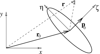
Figure 1: Particle-fixed frame of reference at time $t=0$.

The $(\zeta,\eta)$ system of coordinates is chosen with its origin at the center of the wave packet, ${\bf{r}}_{0}$, and $\zeta$-axis pointing in the direction of ${\bf{p}}_{0}$, with $\eta$-axis perpendicular to ${\bf{p}}_{0}$:

$${\bf{r}}={\bf{r}}_{0}+{\bf U}_{0}\left(\begin{array}[]{c}\zeta\\ \eta\end{array}\right),$$ (4)

where ${\bf U}_{0}$ is a $2\times 2$ real matrix relating the two coordinate systems, see Fig. 1.

When the wave packet is far from any scatterers, its time propagation is dominated by free streaming, described by the propagator

$$G_{\mathrm{fs}}({\bf{r}},{\bf{r}}^{\prime},t)=\left(\frac{m}{2\pi i\hbar t}\right)^{d/2}\exp{\frac{im}{2\hbar t}({\bf{r}}-{\bf{r}}^{\prime})^{2}},$$ (5)

where $m$ is the mass of the moving particle, and $d=2$. Application of this propagator to the wave function given by Eq. (3) yields, up to an irrelevant phase factor, a new Gaussian wave packet of the form of Eq. (3) with

$$\Omega_{\|0}\rightarrow \Omega_{\|t}=\Omega_{\|0}+i{\lambda\!\!\!\!\,{}^{-}}vt/2$$ (6)

$$\Omega_{0}\rightarrow \Omega_{t}=\Omega_{0}+i{\lambda\!\!\!\!\,{}^{-}}vt/2,$$ (7)

where $v=|{\bf{p}}_{0}|/m$ is the average velocity of the particle. The new particle-fixed frame of reference is related to the stationary one by means of Eq. (4), with the wave packet center, ${\bf{r}}_{0}$, replaced by ${\bf{r}}_{t}={\bf{r}}_{0}+({\bf{p}}_{0}/|{\bf{p}}_{0}|)vt$ and ${\bf U}_{t}={\bf U}_{0}$. The average momentum of the wave packet stays unaffected: ${\bf{p}}_{t}={\bf{p}}_{0}$.

To find the semi-classical propagator describing a collision of the particle with one scatterer, we start with the general expression for the semi-classical propagator as a sum of terms of the form brbh

$$\begin{split}G_{\mathrm{sc}}({\bf{r}},{\bf{r}}^{\prime},t)=&\left(\frac{1}{2\pi i\hbar}\right)^{d/2}|D|^{1/2}\\ &\times\exp{\>i\!\left(\frac{S({\bf{r}},{\bf{r}}^{\prime},t)}{\hbar}+\frac{\pi\mu}{2}\right)},\end{split}$$ (8)

where $S({\bf{r}},{\bf{r}}^{\prime},t)$ is the classical action along a classical path from ${\bf{r}}^{\prime}$ to ${\bf{r}}$ in time $t$, $\mu$ is an index equal to twice the number of collisions of the particle with hard disk scatterers over time $t$ gasp , $D=\det(-\partial^{2}S/\partial{\bf{r}}\partial{\bf{r}}^{\prime})$, and $d=2$. In general, there are two classical paths connecting points ${\bf{r}}$ and ${\bf{r}}^{\prime}$, assuming that ${\bf{r}}$ is not in the geometric shadow of ${\bf{r}}^{\prime}$: a reflected path and a direct one. The contribution of the direct path from ${\bf{r}}^{\prime}$ to ${\bf{r}}$ to the time evolution of the wave packet is negligible after time $t$ if a classical particle with momentum ${\bf{p}}_{0}$ would collide with the scatterer during the interval $(0,t)$. Thus, we only consider the propagator given by the reflected path.

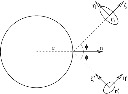
Figure 2: Particle-fixed frames of reference: $(\zeta^{\prime},\eta^{\prime})$ at time $0$ and $(\zeta,\eta)$ at $t$.

Consider a wave packet centered around ${\bf{r}}^{\prime}_{0}$ at time $t=0$ before a collision and around ${\bf{r}}_{0}$ at $t$ after the collision, Fig. 2. The system of reference originates at the point of classical collision. We suppose that the wave-packet to which the propagator will be applied is sufficiently small that we only need to find classical trajectories by minimizing the action for points starting close to ${\bf{r}}^{\prime}_{0}$ and ending close to ${\bf{r}}_{0}$ at time $t$. We then write the action, $S_{\bf R}({\bf{r}}_{0}+\delta{\bf{r}},{\bf{r}}^{\prime}_{0}+\delta{\bf{r}}^{\prime},t)$, for a trajectory from ${\bf{r}}^{\prime}_{0}+\delta{\bf{r}}^{\prime}$, $|\delta{\bf{r}}^{\prime}|\ll|{\bf{r}}^{\prime}_{0}|$, colliding with a scatterer at point ${\bf R}$ and arriving at ${\bf{r}}_{0}+\delta{\bf{r}}$, $|\delta{\bf{r}}|\ll|{\bf{r}}_{0}|$, at time, $t$, as

$$\begin{split}S_{\bf R}&({\bf{r}}_{0}+\delta{\bf{r}},{\bf{r}}^{\prime}_{0}+\delta{\bf{r}}^{\prime},t)\\ &=\frac{m}{2t}\left(\left|{\bf R}-{\bf{r}}^{\prime}_{0}-\delta{\bf{r}}^{\prime}\right|+\left|{\bf{r}}_{0}+\delta{\bf{r}}-{\bf R}\right|\right)^{2}.\end{split}$$ (9)

The variation of this action with respect to the point of collision, ${\bf R}$, leads to an extremum equation that is used to determine the collision point, ${\bf R}$. The algebra simplifies a bit if we take the case where $|{\bf{r}}^{\prime}_{0}|=|{\bf{r}}_{0}|=r$. Using the variational procedure, we find

$$G_{\mathrm{sc}}(\zeta,\eta,\zeta^{\prime},\eta^{\prime},t)=G_{\mathrm{sc}}^{(1)}(\zeta,\zeta^{\prime},t)G_{\mathrm{sc}}^{(2)}(\eta,\eta^{\prime},t),$$ (10)

with

$$G_{sc}^{(1)}(\zeta,\zeta^{\prime},t)\approx\left(\frac{1}{4\pi i{\lambda\!\!\!\!\,{}^{-}}r}\right)^{1/2}\exp{\frac{i(\zeta+2r-\zeta^{\prime})^{2}}{4{\lambda\!\!\!\!\,{}^{-}}r}}$$ (11)

and

$$\begin{split}G_{sc}^{(2)}&(\eta,\eta^{\prime},t)\approx\left(\frac{a\cos\phi}{4\pi i{\lambda\!\!\!\!\,{}^{-}}r(r+a\cos\phi)}\right)^{1/2}\\ &\times\exp{\frac{ia(\eta-\eta^{\prime})^{2}\cos\phi+2ir(\eta^{2}+(\eta^{\prime})^{2})}{4{\lambda\!\!\!\!\,{}^{-}}r(r+a\cos\phi)}}.\end{split}$$ (12)

Here $\eta,\zeta$ and $\eta^{\prime},\zeta^{\prime}$ are coordinates with origins at ${\bf{r}}_{0}$ and ${\bf{r}}^{\prime}_{0}$ respectively, such that $\zeta,\zeta^{\prime}$ are along the direction of the probability current, and $\eta,\eta^{\prime}$ are in directions perpendicular to $\zeta,\zeta^{\prime}$, respectively, as illustrated in Fig. 2. Further, $\phi$ is the angle of incidence in the collision. The time dependence in the propagator appears in $r$, through the relation $2r=vt$.

There are limits to the range of applicability of the semi-classical propagator given by Eq. (10). First, the particle’s wave function is supposed to be confined to a small region in space, the linear size of which is much smaller that the radius of the scatterer, throughout the time interval $(0,t)$. It is this limitation that allows one to consider only the reflected path while deriving the propagator. Second, the wave packet size is assumed to be much smaller than the distance $r$ between the center of the wave packet and the point where the particle would, classically, collide with the scatterer. This assumption makes it possible to expand the coordinates of points connected by the propagator about corresponding wave packet centers.

The propagator in the direction of motion given by Eq. (11) is simply the free streaming expressed in particle-fixed coordinate frames, showing that time evolution of $\zeta$-component of the time dependent wave packet, $\psi_{t}$, is unaffected by scattering events. The $\eta$-component of the propagator, Eq. (12), can be easily shown to satisfy the identity

$$\begin{split}G_{\mathrm{sc}}^{(2)}(\eta,\eta^{\prime},t)=\int d\eta_{1}&\int d\eta_{2}\>G_{\mathrm{fs}}(\eta,\eta_{2},t/2)\\ &\times\hat{C}(\eta_{2},\eta_{1})G_{\mathrm{fs}}(\eta_{1},\eta^{\prime},t/2),\end{split}$$ (13)

where we introduced an instantaneous collision propagator, $\hat{C}(\eta,\eta^{\prime})$, according to

$$\hat{C}(\eta,\eta^{\prime})=\delta(\eta-\eta^{\prime})\exp\frac{i\eta^{2}}{{\lambda\!\!\!\!\,{}^{-}}a\cos\phi}.$$ (14)

Eq. (13) allows to represent the propagator for a single scattering event, $G_{\mathrm{sc}}(\zeta,\eta,\zeta^{\prime},\eta^{\prime},t)$, as a product of three successive propagators: (i) a free streaming propagator, $G_{\mathrm{fs}}(\zeta_{1},\eta_{1},\zeta^{\prime},\eta^{\prime},t/2)$, (ii) an instantaneous collision propagator, $\delta(\zeta_{2}-\zeta_{1})\hat{C}(\eta_{2},\eta_{1})$ affecting the $\eta$-component of $\psi_{t}$, and (iii) another free streaming propagator, $G_{\mathrm{fs}}(\zeta,\eta,\zeta_{2},\eta_{2},t/2)$.

Assuming that the wave packet size $\sigma_{t}$ remains smaller than radius $a$ of a scatterer, over the time $t$, we now construct the propagator for a trajectory with several collisions of the moving particle with scatterers as a combination of free particle and single collision propagators. This is appropriate in the semi-classical approximation when the size of the wave packet is small compared to the size of a scatterer, and to the average separation of the scatterers. Both free flight and instantaneous collision propagators leave the Gaussian form of a wave packet invariant. While the effect of the free streaming is described by Eqs. (6, 7), the instantaneous collision propagator, Eq. (14), when applied to a Gaussian wave packet leads to an instantaneous change in $\Omega$ given by

$$\frac{1}{\Omega^{+}}=\frac{1}{\Omega^{-}}-\frac{4i}{{\lambda\!\!\!\!\,{}^{-}}a\cos\phi},$$ (15)

where superscripts $\pm$ are used to distinguish variables immediately before and immediately after a collision. As mentioned above, $\Omega_{\|}$ is unaffected by instantaneous collisions: $\Omega_{\|}^{+}=\Omega_{\|}^{-}$.

The free streaming transformation of $\Omega_{t}$, coupled with the collisional transformation of $\Omega^{-}$ to $\Omega^{+}$ given above provides a direct connection between this semi-classical analysis of wave packet motion and the method of Sinai et al. for analyzing the ergodic properties of the classical Lorentz gas in terms of the curvature of a classical wave front sinai ; vbd . In fact a simple transformation allows us to recover the classical equations, and to identify the appearance of the positive Lyapunov exponent in the semi-classical formulae. To see this let us define complex radii of curvature, $\tilde{\rho}_{\|}$ and $\tilde{\rho}$, according to

$$\Omega_{\|}=\frac{i}{2}{\lambda\!\!\!\!\,{}^{-}}\tilde{\rho}_{\|}\;\;\;\;\;\mathrm{and}\;\;\;\;\;\Omega=\frac{i}{2}{\lambda\!\!\!\!\,{}^{-}}\tilde{\rho}.$$ (16)

In terms of $\tilde{\rho}$, Eqs. (7 and 15) read

$$\tilde{\rho}_{t}=\tilde{\rho}_{0}+vt \mathrm{free\>\>streaming,}$$ (17)

$$\displaystyle\frac{1}{\tilde{\rho}^{+}}=\frac{1}{\tilde{\rho}^{-}}+\frac{2}{a\cos\phi} \mathrm{collision,}$$ (18)

while $\tilde{\rho}_{\|t}=\tilde{\rho}_{\|0}+vt$ regardless of whether any scattering events have taken place over time $t$. These equations for $\tilde{\rho}$ are identical with the curvature equations sinai for the classical Lorentz gas. In an unpublished manuscript describing the diffractive scattering of a wave packet by a circular scatterer, Wirzba wirz noted that the curvature equations can also be extracted from his formalism.

To describe the spreading of a Gaussian wave packet in the Lorentz gas, we consider a sequence of collisions parameterized by a set of times $\{t_{j}\}$ together with a set of collision angles $\{\phi_{j}\}$. Direct substitution of the free streaming transformation for $\tilde{\rho}_{t}$, Eq. (17), into the expression for the size of the wave packet along the $\eta$-coordinate, i.e. along the direction perpendicular to the average momentum ${\bf{p}}$ of the particle, $\sigma_{t}^{2}=1/\>{\mathcal{R}}\!e\!\>(\Omega_{t}^{-1})={\lambda\!\!\!\!\,{}^{-}}/(2\>{\mathcal{I}}\!m\!\>(\tilde{\rho}_{t}^{-1}))$, yields

$$\sigma_{t}=\sigma_{t_{j}}\left|\frac{\tilde{\rho}_{t_{j}}+v(t-t_{j})}{\tilde{\rho}_{t_{j}}}\right|=\sigma_{t_{j}}\exp{\left(v\>{\mathcal{R}}\!e\!\int_{t_{j}}^{t}\frac{d\tau}{\tilde{\rho}_{\tau}}\right)},$$ (19)

for $t_{j}<t<t_{j+1}$. It follows from the relation between $\sigma$ and $\tilde{\rho}$, and the change in $\tilde{\rho}$ on collision, that the instantaneous scattering transformation does not change the size of the wave packet $(\sigma_{t_{j}}^{+}=\sigma_{t_{j}}^{-})$. Thus, we can propagate $\sigma_{t}$ backward in time to get

$$\sigma_{t}=\sigma_{0}\exp{\left(v\>{\mathcal{R}}\!e\!\int_{0}^{t}\frac{dt^{\prime}}{\tilde{\rho}_{t^{\prime}}}\right)}=\sigma_{0}\>e^{t\lambda_{t}},$$ (20)

where $\sigma_{0}$ is the initial size of the wave packet at $t=0$, and

$$\lambda_{t}=\frac{v}{t}\>{\mathcal{R}}\!e\!\int_{0}^{t}\frac{d\tau}{\tilde{\rho}_{\tau}}=\frac{v}{t}\int_{0}^{t}\frac{d\tau}{\rho_{\tau}},$$ (21)

where we introduce a real radius of curvature, $\rho$, as

$$1/\rho\equiv\>{\mathcal{R}}\!e\!\;(1/\tilde{\rho}).$$ (22)

The quantity $\lambda_{t}$ can be thought of as a wave packet stretching exponent over a time $t$. It differs from the classical Lyapunov exponent $\lambda$ because it contains quantum effects and the limit of infinite time is not taken. The stretching exponent, $\lambda_{t}$, converges to the Lyapunov exponent, $\lambda$, in the long time classical limit:

$$\lim_{t\rightarrow\infty}\lim_{{\lambda\!\!\!\!\,{}^{-}}\rightarrow 0}\lambda_{t}=\lambda.$$ (23)

In order to prove Eq. (23), one needs to show that $\rho$ becomes the classical radius of curvature for the classical Lorentz gas as ${\lambda\!\!\!\!\,{}^{-}}\rightarrow 0$. Substituting Eq. (22) along with $\>{\mathcal{I}}\!m\!\>(1/\tilde{\rho})={\lambda\!\!\!\!\,{}^{-}}/(2\sigma^{2})$ into the transformations for $\tilde{\rho}_{t}$, Eqs. (17, 18), one gets

$$\left.\begin{array}[]{ccl}\rho_{t}&=&\displaystyle\frac{(\rho_{0}+vt)^{2}+\varepsilon_{0}(vt)^{2}}{\rho_{0}+vt+\varepsilon_{0}vt}\\ &&\\ \sigma_{t}&=&\displaystyle\frac{\sigma_{0}}{\rho_{0}}\sqrt{(\rho_{0}+vt)^{2}+\varepsilon_{0}(vt)^{2}}\end{array}\right\}\;\;\;\mathrm{free\>\>streaming,}$$ (24)

and $1/\rho^{+}=1/\rho^{-}+2/(a\cos\phi)$ together with $\sigma^{+}=\sigma^{-}$ at a collision. Here

$$\varepsilon_{t}=\left(\frac{{\lambda\!\!\!\!\,{}^{-}}\rho_{t}}{2\sigma_{t}^{2}}\right)^{2}$$ (25)

contains all the quantum effects; it vanishes as ${\lambda\!\!\!\!\,{}^{-}}\rightarrow 0$, which makes Eq. (24) converge to its classical counterpart sinai ; vbd . Another way to visualize the semi-classical corrections is to rewrite Eq. (24) in differential form:

$$\dot{\rho}_{t}=v(1-\varepsilon_{t})\;\;\;\;\;\mathrm{and}\;\;\;\;\;\dot{\sigma}_{t}=v\sigma_{t}/\rho_{t}.$$ (26)

Here the second equation has its classical form, and the quantum correction is apparent in the first equation: it shows that the free flight spreading of the wave packet results from a combination of a classical linear separation of trajectories and the quantum spreading due to the Uncertainty Principle.

The role of the Uncertainty Principle becomes apparent from the following simple consideration. Suppose one prepares a tiny minimal wave packet with spatial uncertainty $\sigma_{0}$. The corresponding uncertainty in momentum, $\Delta p$, is then given by $\sigma_{0}\Delta p=\hbar/2$. After some time $t$ the wave packet size evolves to $\sigma_{\mathrm{UP}}\approx(\Delta p/m)t={\lambda\!\!\!\!\,{}^{-}}vt/(2\sigma_{0})$ merely due to the Uncertainty Principle. Writing the geometrical (classical) spreading as $\sigma_{\mathrm{CL}}=\sigma_{0}(1+vt/\rho_{0})$, we notice that $\sigma_{t}$ in Eq. (24) is essentially a simple combination of $\sigma_{\mathrm{CL}}$ and $\sigma_{\mathrm{UP}}$, namely $\sigma_{t}=\sqrt{\sigma_{\mathrm{CL}}^{2}+\sigma_{\mathrm{UP}}^{2}}$.

Figure 3: Free flight time evolution of $\rho$ and $\sigma$: (a) classical case, $\varepsilon=0$, (b) quantum case, $\varepsilon>0$.

Fig. 3 illustrates the free flight dynamics of $\rho$ and $\sigma$ given by Eq. (26). Fig. 3(a) pictures the classical limit, ${\lambda\!\!\!\!\,{}^{-}}=0$: an arc of instantaneous radius $\rho$ and length $\sigma$ moves with constant velocity $v$ along the “cone” originating at a point $O$. Eq. (26) with $\varepsilon_{t}=0$ describes the time evolution of $\rho$ and $\sigma$ in this case. In quantum regime, $\varepsilon>0$, the point $O$ is also moving in the same direction as the arc, but with a different, time dependent, velocity equal to $\varepsilon v$, see Fig. 3(b). It can be shown from Eqs. (25, 26) that $\varepsilon_{t}\sim t^{-2}$ as $t\rightarrow\infty$, implying the convergence of point $O$ to some point $O^{\prime}$ in the long time limit, see Fig. 3(b). The time evolution of $\rho$ and $\sigma$ is then dominated by classical equations when $O$ is close to $O^{\prime}$.

We now define an interval of time, called the Lyapunov regime for which the values of $\rho$ and $\sigma$ satisfy the inequality $\varepsilon\ll 1$. It follows from the free flight and collision transformations for $\rho_{t}$ and $\sigma_{t}$ that $\varepsilon_{t}$ is a rapidly decreasing function of time, see Fig. 4. Therefore, once in the Lyapunov regime the system stays in it for some time $t_{L}$, at which $\sigma$ becomes comparable with the size of scatterers, and our collision analysis breaks down. It can also be shown that if the Lyapunov regime inequality is not satisfied at $t=0$, and the wave packet is small, the system rapidly evolves to a state for which this inequality is satisfied. During this transient regime $\rho$ rapidly decreases whereas $\sigma$ does not change significantly, see Fig. 4.

In the Lyapunov regime, the first equation in Eqs. (26) reduces to its classical counterpart, $\dot{\rho}\approx v$, so that $\sigma_{t}$ grows exponentially in the same way as a small pencil of trajectories separates exponentially in the classical system. That is $\sigma_{t}=\sigma_{0}\exp{(t\lambda_{t})}$, where $\lambda_{t}$ is given by Eq. (21) and calculated using only classical mechanics. It is useful to remark that $\lambda_{t}$ typically reaches a value close to the classical Lyapunov exponent $\lambda$ after only a few collisions, see Fig. 4. On the other hand, one can estimate that the upper limit of $t_{L}$, the maximum duration of the Lyapunov regime, is $t_{L}^{\mathrm{m}ax}\sim(1/(2\lambda))\ln(a/{\lambda\!\!\!\!\,{}^{-}})$, that is, about half of the Ehrenfest time haake , which for sufficiently small ${\lambda\!\!\!\!\,{}^{-}}$ can be long enough for the wave packet to exhibit exponential spreading.

Finally, we illustrate the exponential spreading of a Gaussian wave packet for the case of particles moving in short, periodic orbits. We numerically evaluate $\sigma_{t}$ and $\rho_{t}$ in Eq. (26) (and in the $\rho^{-}$ to $\rho^{+}$ collision transformation) for the simplest periodic orbit: a particle moving back and forth along the line connecting the centers of two disks. Fig. 4 shows $\sigma_{t}$, $\rho_{t}$, and quantity $\varepsilon_{t}$, given by Eq. (25), for the two disks of radius $a=1$, and the center-to-center separation $R=3$. The particle is placed in the middle between the two disks at $t=0$, and has the de Broglie wavelength ${\lambda\!\!\!\!\,{}^{-}}=10^{-7}$. The initial wave packet is characterized by $\sigma_{0}=2\cdot 10^{-4}$ and $\rho_{0}=10$, so that $\varepsilon_{0}\approx 156$ and the system is far from the Lyapunov regime at $t=0$. Fig. 4 shows that it only takes a single collision for the system to reach the Lyapunov regime, $\varepsilon\ll 1$.

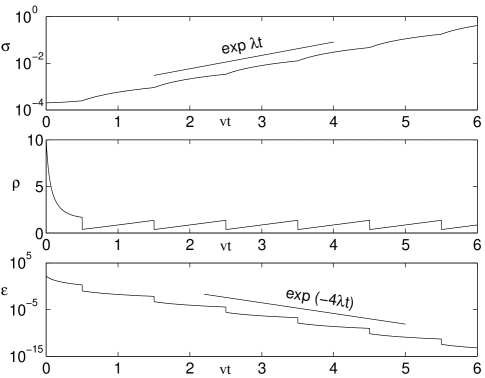
Figure 4: Wave packet size, $\sigma$, real radius of curvature, $\rho$, and $\varepsilon$, are shown as functions of time, $t$, for a two-disk periodic orbit. Disk radii $a=1$, center-to-center separation $R=3$, de Broglie wave length ${\lambda\!\!\!\!\,{}^{-}}=10^{-7}$. The corresponding Lyapunov exponent $\lambda/v\approx 1.32$. Initial wave packet size $\sigma_{0}=2\cdot 10^{-4}$ and $\rho_{0}=10$. The particle is located in the middle between the two disks at $t=0$. Exponential trends are shown for plots of $\sigma$ and $\varepsilon$. All distances are measured in units of $a$.

The parameters in Fig. 4 are chosen so as to illustrate the essential regimes: a short decay of quantum effects ($\varepsilon$ becomes less than unity), followed by the Lyapunov spreading of the wave packet, $\sigma\sim\exp(\lambda t)$. The relatively small value of the de Broglie wavelength used in this example can be indeed achieved experimentally exper .

The classical Lyapunov exponent of a two-disk periodic orbit is known exactly jose ; gaspbk ,

$$\lambda=\frac{v}{R-2a}\ln\frac{R-a+\sqrt{R(R-2a)}}{a}.$$ (27)

In our case Eq. (27) gives $\lambda/v\approx 1.32$. The numerical evaluation presented in Fig. 4 shows that a single collision is enough to initiate the exponential growth of the wave packet (with the rate given by the classical Lyapunov exponent), which persists for about 5-6 collisions. Our results do not apply for times longer than the duration of the Lyapunov regime, $vt_{L}/a\approx 6$.

III The wave-packet auto-correlation function

As an application of the analysis of wave packet dynamics developed above, we calculate the wave packet auto-correlation function, $C(t)$, defined in Eq. (1), for particles moving in periodic orbits. Here the initial state, $|0\rangle$, describes a Gaussian wave packet centered about ${\bf{r}}_{0}$ with its average momentum ${\bf{p}}_{0}$, such that the phase point $({\bf{r}}_{0},{\bf{p}}_{0})$ lies on a periodic orbit of the corresponding classical system. The auto-correlation function for periodic orbits in billiard systems was studied by Heller heller some time ago using different techniques. The calculations presented here agree with Heller’s results and provide some additional information about this correlation function.

The reasons for restricting our calculations to periodic orbits are as follows. The expansion used above to obtain the semi-classical single collision propagator in the previous section, Eq. (10), is correct for wave packets which are small compared to disk radii and average separation among scatterers. Mathematically, this limitation is a consequence of the truncation of the expansion of the coordinates of starting and final points connected by the propagator, ${\bf{r}}^{\prime}$ and ${\bf{r}}$ respectively, about the centers of initial and final wave packets respectively, i.e. ${\bf{r}}^{\prime}={\bf{r}}^{\prime}_{0}+\delta{\bf{r}}^{\prime}$ and ${\bf{r}}={\bf{r}}_{0}+\delta{\bf{r}}$. Therefore, one gets a close approximation to the particle’s wave function at positions close to the wave packet center, ${\bf{r}}_{0}$, but the approximation may fail on the periphery of the wave packet. Our calculations of the auto-correlation function, $C(t)$, or Loschmidt echo, $M(t)$, are only reliable when the relevant overlap integrals are dominated by central region of the wave function, and contributions coming from wave packet wings can be neglected. This condition is most easily satisfied when the classical motion is along a periodic orbit. The result for the decay of the Loschmidt echo reported earlier gd , as $\exp(-2\lambda t)$, is incorrect because this restriction on the validity of the semi-classical approximation was not properly taken into account. This error first became apparent when we obtained an exact result that is inconsistent with this decay. The exact result is described in the next section.

Figure 5: A Gaussian wave packet is shown at time $t=0$ (centered about point $O$), and at a later time $t=nT+\Delta/v$ (centered about point $P$). Points $O$ and $P$ lie on the same periodic orbit, and are separated in time by $n$ ($=0,1,2,\ldots,N$) periods, $T$, of the periodic orbit, plus a short time interval $\Delta/v$. The separation distance $\Delta$ is assumed to be sufficiently small in order for the initial and final wave packets to overlap significantly.

Consider a wave packet whose initial average coordinate, ${\bf{r}}_{0}$, and momentum, ${\bf{p}}_{0}$, correspond to a phase space point on a periodic orbit, with period $T$, of the classical Lorentz gas. Suppose that $nT$ is smaller than the Ehrenfest time, for $n=0,1,2,\ldots,N$ so that we can apply the analysis developed in the previous section in order to propagate the wave packet over times

$$t=nT+\Delta/v,$$ (28)

where the displacement $\Delta$ is sufficiently small in order for the initial and final wave packets to overlap significantly, as illustrated in Fig. 5. For simplicity we take the initial wave function, $\psi_{0}$, to be a “circular” wave packet, i.e. $\sigma_{\|0}=\sigma_{0}$ and $\rho_{\|0}=\rho_{0}$ with the explicit form,

$$\begin{split}\psi_{0}&(x,y)=\left(\frac{1}{2\pi\sigma_{0}^{2}}\right)^{1/2}\\ &\times\exp\left[-\frac{1}{4}\left(\frac{1}{\sigma_{0}^{2}}-\frac{2i}{{\lambda\!\!\!\!\,{}^{-}}\rho_{0}}\right)(x^{2}+y^{2})+\frac{i}{{\lambda\!\!\!\!\,{}^{-}}}x\right],\end{split}$$ (29)

where $x$-axis is directed along ${\bf{p}}_{0}$. In the same coordinate system the wave packet $\psi_{t}$ propagated from $\psi_{0}$ over time $t$, given by Eq. (28), reads, up to an irrelevant phase factor,

$$\begin{split}\psi_{t}(x,y)=&\left(\frac{1}{2\pi\sigma_{\|}\sigma}\right)^{1/2}\exp\left[-\frac{1}{4}\left(\frac{1}{\sigma_{\|}^{2}}-\frac{2i}{{\lambda\!\!\!\!\,{}^{-}}\rho_{\|}}\right)(x-\Delta)^{2}\right.\\ &\left.-\frac{1}{4}\left(\frac{1}{\sigma^{2}}-\frac{2i}{{\lambda\!\!\!\!\,{}^{-}}\rho}\right)y^{2}+\frac{i}{{\lambda\!\!\!\!\,{}^{-}}}(x-\Delta)\right].\end{split}$$ (30)

Here, $\sigma_{\|}$, $\sigma$, $\rho_{\|}$ and $\rho$ depend on time $t$ through a sequence of free flight and collision transformations developed in the previous section. The probability distribution $|\psi_{0}({\bf{r}})|^{2}$ is negligible outside a small circle of radius $r\sim\sigma_{0}$. Therefore, the main contribution to the overlap $\langle\psi_{0}|\psi_{t}\rangle$ comes from the points inside this circle, and the central regions of the wave packets will dominate the integrals for small center-to-center separations $\Delta$, as illustrated in Fig. 5.

A straightforward calculation shows that for $t$ given by Eq. (28)

$$C(t)=\left|\int d{\bf{r}}\>\psi_{0}^{*}({\bf{r}})\psi_{t}({\bf{r}})\right|^{2}=\frac{A}{\sigma}\exp(-\alpha\Delta^{2}),$$ (31)

where

$$A = \frac{4}{\sigma_{0}^{2}}\left|\frac{g_{\|}g}{\sigma_{\|}}\right|,$$ (32)

$$\alpha = \frac{1}{2}\>{\mathcal{R}}\!e\!\left[g_{\|}\left(\frac{1}{\sigma_{\|}^{2}}-\frac{2i}{{\lambda\!\!\!\!\,{}^{-}}\rho_{\|}}\right)\left(\frac{1}{\sigma_{0}^{2}}+\frac{2i}{{\lambda\!\!\!\!\,{}^{-}}\rho_{0}}\right)\right],$$ (33)

with

$$\begin{split}g&\equiv\left[\frac{1}{\sigma^{2}}+\frac{1}{\sigma_{0}^{2}}-\frac{2i}{{\lambda\!\!\!\!\,{}^{-}}}\left(\frac{1}{\rho}-\frac{1}{\rho_{0}}\right)\right]^{-1},\\ g_{\|}&\equiv\left[\frac{1}{\sigma_{\|}^{2}}+\frac{1}{\sigma_{0}^{2}}-\frac{2i}{{\lambda\!\!\!\!\,{}^{-}}}\left(\frac{1}{\rho_{\|}}-\frac{1}{\rho_{0}}\right)\right]^{-1}.\end{split}$$ (34)

As seen from Eq. (31) the auto-correlation function exhibits a sequence of peaks corresponding to partial reconstruction of the wave packet at times $t=nT$. These peaks, first studied by Heller heller , have a simple physical origin: the wave packet repeatedly passes through the starting point giving rise to strong maxima of the return probability $C(t)$. These maxima are periodic orbit revivals and should be distinguished from more general classes of quantum revivals that do not require a particular periodic orbit for their appearance toms . It can be shown that time dependence of $A$ and $\alpha$ is sub-exponential compared to to the exponential growth of $\sigma$ with time, so that the periodic orbit revival peaks have predominantly Gaussian form. The strength of the peaks decreases exponentially with time with a rate given by the Lyapunov exponent of the periodic orbit. This follows from the fact that height of the peaks is mainly determined by the exponential growth of the size of a wave packet, $\sigma\sim\exp(\lambda t)$. It is worth noting that $A$ decays with time in a power law manner making the auto-correlation function to decay slightly faster than $\exp(-\lambda t)$, see Fig. 6.

Fig. 6 shows the numerical evaluation of the revivals in Eq. (31) for the two-disk periodic orbit described in previous section, see Fig. 4. A particle of the de Broglie wavelength ${\lambda\!\!\!\!\,{}^{-}}=10^{-7}$ moves back and forth between two disks of radii $a=1$, with the center-to-center separation $R=3$, along the line connecting the centers. The initial wave packet is located in the middle between the two disks, and is characterized by $\sigma_{\|0}=\sigma_{0}=2\cdot 10^{-4}$ and $\rho_{\|0}=\rho_{0}=10$. The left part of Fig. 6 shows the revival maxima $C_{\mathrm{max}}$, which occur at $t_{\mathrm{max}}=nT$. The right part shows the auto-correlation function in small neighborhoods of the corresponding maxima.

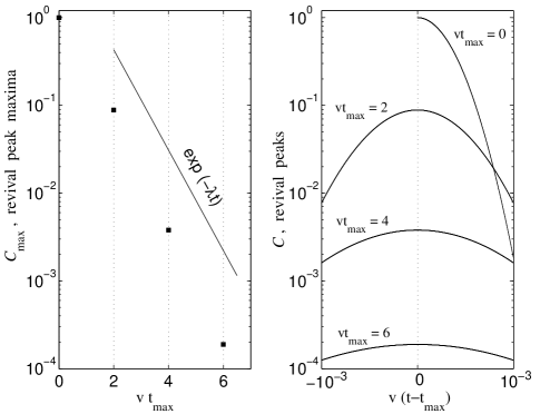
Figure 6: Revival peaks of the wave packet auto-correlation function, $C(t)$, for the same two-disk periodic orbit as in Fig. 4: $a=1$ and $R=3$. Particles de Broglie wave length ${\lambda\!\!\!\!\,{}^{-}}=10^{-7}$. The initial wave packet is characterized by $\sigma_{0}=\sigma_{\|0}=2\cdot 10^{-4}$ and $\rho_{0}=\rho_{\|0}=10$. The exponential trend is indicated by a straight line.

It easy to show that in case of the two-disk periodic orbit, the revival peaks are separated by deep minima of the auto-correlation function. The minima occur when the average momenta of the original wave packet and the one propagated in time $t$ are pointing in opposite directions. When this happens, $\psi_{0}$ and $\psi_{t}$ interfere destructively, and the auto-correlation integral, $C(t)$, is very small. We calculate the overlap of $\psi_{0}$ and $\psi_{t}$ at $t=(n+1/2)T$, when the two wave packets are centered about the same point, but move in opposite directions. The initial wave function is given by Eq. (29), while

$$\begin{split}\psi_{t}(x,y)=&\left(\frac{1}{2\pi\sigma_{\|}\sigma}\right)^{1/2}\exp\left[-\frac{1}{4}\left(\frac{1}{\sigma_{\|}^{2}}-\frac{2i}{{\lambda\!\!\!\!\,{}^{-}}\rho_{\|}}\right)x^{2}\right.\\ &\phantom{aaaaaaaaa}\left.-\frac{1}{4}\left(\frac{1}{\sigma^{2}}-\frac{2i}{{\lambda\!\!\!\!\,{}^{-}}\rho}\right)y^{2}-\frac{i}{{\lambda\!\!\!\!\,{}^{-}}}x\right].\end{split}$$ (35)

Then,

$$C(t)=\left|\int d{\bf{r}}\>\psi_{0}^{*}({\bf{r}})\psi_{t}({\bf{r}})\right|^{2}=\frac{A}{\sigma}\exp\left(-\frac{2}{{\lambda\!\!\!\!\,{}^{-}}^{2}}\>{\mathcal{R}}\!e\!\;g_{\|}\right),$$ (36)

where $A$ and $g_{\|}$ are defined in Eqs. (32, 34). It can be shown that the exponential in Eq. (36) is a very small number if the condition ${\lambda\!\!\!\!\,{}^{-}}\ll\sigma_{0},\rho_{0}$ is satisfied, e.g. in case of the periodic orbit considered above (Fig. 4 and Fig. 6) $\>{\mathcal{R}}\!e\!\;g_{\|}$ ranges from $2\cdot 10^{-8}$ to $4\cdot 10^{-8}$ making $C(t)$ smaller than $(A/\sigma)\exp(-4\cdot 10^{6})$, which is practically zero when compared with values of $C(t)$ at the PO revival maxima.

Similar deep minima of the auto-correlation function will occur for particles in more complicated periodic orbits, making the revivals very pronounced.

IV A simple hard sphere Loschmidt echo

Having described the wave-packet auto-correlation function for the Lorentz gas, we now present a simple identity that allows us to use this correlation function to calculate, analytically, the Loschmidt echo for a very particular perturbation. The Loschmidt echo was defined by Eq. (2). We suppose that the perturbed Hamiltonian is obtained from the unperturbed one by changing the mass of the moving particle, from $m$ to $m+\delta m$. The identity depends on the fact that for hard scatterers, no matter what their shape, the eigenfunctions depend on wave numbers rather than on the mass of the moving particle. That is, the sets of eigenfunctions for particles of different masses are the same, only the values of the energy corresponding to the same wave numbers differ. The wave functions are the solutions of the scalar Helmholtz equation

$$\left(\nabla^{2}+k^{2}\right)\phi_{\bf{k}}({\bf{r}})=0$$ (37)

which satisfy the Dirichlet boundary condition that $\phi_{\bf{k}}({\bf{r}})$ vanishes on the surface of each scatterer, and on the boundaries of the system.

We can express the time propagator for a moving particle of mass $m$ under a Hamiltonian $H_{m}$ as

$$\exp\left(-\frac{it}{\hbar}H_{m}\right)=\sum_{\bf{k}}|\phi_{\bf{k}}\rangle\exp\left(-\frac{i\hbar t}{2m}k^{2}\right)\langle\phi_{\bf{k}}|,$$ (38)

where the summation is over all possible eigenstates of the system. These eigenstates, $|\phi_{\bf{k}}\rangle$, satisfy an orthonormality relation

$$\langle\phi_{{\bf{k}}^{\prime}}|\phi_{\bf{k}}\rangle=\delta_{{\bf{k}}^{\prime},{\bf{k}}},$$ (39)

where the choice between Kronecker and Dirac delta functions is dictated by the nature of the eigenstates. Eqs. (38, 39) hold for systems with hard wall potentials in any number of spatial dimensions.

This representation of the time displacement operator, Eq. (38), together with the orthonormality condition, Eq. (39), leads to the following identity

$$\exp\left(\frac{it}{\hbar}H_{m+\delta m}\right)\exp\left(-\frac{it}{\hbar}H_{m}\right)=\exp\left(-\frac{it_{s}}{\hbar}H_{m}\right),$$ (40)

where $t_{s}$ is a scaled time, related to the physical time $t$ by

$$t_{s}=\frac{\delta m}{m+\delta m}t.$$ (41)

This identity permits us to express the Loschmidt echo, for this special perturbation, in terms of the wave-packet auto-correlation function as

$$\begin{split}M(t)=\left|\langle 0|\exp\left(\frac{it}{\hbar}H_{m+\delta m}\right)\exp\left(-\frac{it}{\hbar}H_{m}\right)|0\rangle\right|^{2}&\\ =\left|\langle 0|\exp\left(-\frac{it_{s}}{\hbar}H_{m}\right)|0\rangle\right|^{2}=C(t_{s})&.\end{split}$$ (42)

This is the main result of this section. For small perturbations, $\delta m/m\ll 1$, the Loschmidt echo for long times can be expressed in terms of the short time auto-correlation function.

The physical origin of this result is straightforward. Classically, the perturbed and unperturbed masses follow exactly the same trajectory, but with different velocities. Hence the forward motion with mass $m$ followed by the reversed motion with mass $m+\delta m$ has a final position which is different from the initial position, and corresponds to motion over the part of the path that is not reached by the time reversed trajectory. This is exactly reflected by the operator identity, Eq. (40). Perhaps the most remarkable thing about this result is the fact that although for long times a small wave packet will spread over large distances, the Loschmidt echo in this case is determined by the short time spreading of the wave packet, even if the physical time is quite large. As mentioned in Section III, the exact result, Eq. (42), is inconsistent with the Lyapunov decay reported earlier gd .

As discussed in Section III, the auto-correlation function $C(t)$ exhibits a sequence of sharp revival maxima when the particle moves on a classically periodic orbit. The maxima occur at times $t_{\mathrm{max}}$ multiple of the period $T$ of the periodic orbit, and $C(t_{\mathrm{max}})\sim\exp(-\lambda t_{\mathrm{max}})$, where $\lambda$ is the corresponding classical Lyapunov exponent. According to Eq. (42) the mass perturbation Loschmidt echo $M$ at time $t$ is simply the auto-correlation function $C$ at the scaled time $t_{s}$ given by Eq. (41). Thus like the auto-correlation function, the Loschmidt echo $M(t)$ exhibits a periodic sequence of maxima at times

$$t^{\prime}_{\mathrm{max}}=\frac{m+\delta m}{\delta m}t_{\mathrm{max}}=n\frac{m+\delta m}{\delta m}T,$$ (43)

where $n=1,2,\ldots,N$, such that $NT$ is smaller than the duration of the Lyapunov regime, $t_{L}$. The envelope of the maxima exhibits a mainly exponential decay:

$$M(t^{\prime}_{\mathrm{max}})=C(t_{\mathrm{max}})\sim\exp(-\lambda t_{\mathrm{max}})=\exp(-\lambda_{s}t^{\prime}_{\mathrm{max}}).$$ (44)

Here we introduced a scaled Lyapunov exponent according to

$$\lambda_{s}=\frac{\delta m}{m+\delta m}\lambda.$$ (45)

It is important to note that the behavior of the Loschmidt echo described by Eq. (44) can persist for times much longer than $t_{L}$ (for sufficiently small $\delta m$) despite the fact that the analysis of the wave packet dynamics presented in Section II is valid only for times shorter than $t_{L}$.

The Hamiltonian perturbation used in this section is rather trivial since the perturbed Hamiltonian commutes with the unperturbed Hamiltonian. Therefore the results of this section are not to be compared with those obtained for more complicated perturbations such as distortion of the mass tensor past ; cucc .

V Generalization to three dimensions

The derivation of the wave packet propagator in Section II, and the calculation of the periodic orbit revivals, Section III, were carried out for hard-disk systems in two dimensions, $d=2$. We now generalize these calculations to the three dimensional case, $d=3$, using methods similar to those used to describe the classical separation of close trajectories sinai ; vbd

The initial Gaussian wave packet in three dimensions reads

$$\begin{split}\langle{\bf{r}}|0\rangle\equiv\psi_{0}&({\bf{r}})=\left(\frac{1}{2\pi}\right)^{3/4}\left(\frac{1}{\sigma_{\|0}\sigma_{0}^{2}}\right)^{1/2}\\ &\times\exp\left(\frac{i}{{\lambda\!\!\!\!\,{}^{-}}}\zeta-\frac{\zeta^{2}}{4\Omega_{\|0}}-\frac{1}{4}\mbox{\boldmath$\eta$}^{\mathrm{T}}\mbox{\boldmath$\Omega$}_{0}^{-1}\mbox{\boldmath$\eta$}\right),\end{split}$$ (46)

where $\zeta$-axis is directed along the momentum ${\bf{p}}_{0}$, see Fig. 1, while $\mbox{\boldmath$\eta$}\equiv(\eta^{(1)},\eta^{(2)})^{\mathrm{T}}$ lies in the plane perpendicular to ${\bf{p}}_{0}$; $\mbox{\boldmath$\Omega$}_{0}$ is a $2\times 2$ complex symmetric matrix, and $\mathrm{T}$-superscript denotes transposition. As in two-dimensional case, the origin of the orthogonal frame $(\zeta,\eta^{(1)},\eta^{(2)})$ travels with the center of the wavepacket with fixed axes, except at collisions, when the axes rotate so that the new $\zeta$ axis is in the direction of motion of the center of the wave packet, see Fig. 1. The wave packet size in $\zeta$-direction $\sigma_{\|0}^{2}=1/\>{\mathcal{R}}\!e\!\>(\Omega_{\|0}^{-1})$, while in $\eta$-plane

$$\sigma_{0}^{2}=\frac{1}{\sqrt{\det\>{\mathcal{R}}\!e\!\>(\mbox{\boldmath$\Omega$}_{0}^{-1})}}.$$ (47)

Application of the free streaming propagator $G_{\mathrm{fs}}({\bf{r}},{\bf{r}}^{\prime},t)$, given by Eq. (5) with $d=3$, to the wave function above changes $\mbox{\boldmath$\Omega$}_{0}$ to

$$\mbox{\boldmath$\Omega$}_{t}=\mbox{\boldmath$\Omega$}_{0}+i({\lambda\!\!\!\!\,{}^{-}}vt/2){\bf 1},$$ (48)

where ${\bf 1}$ is the $2\times 2$ unit matrix; the change of the $\zeta$-directional component of the wave packet is the same as in the two-dimensional case, Eq. (6).

The single-sphere scattering propagator is given by Eq. (8) with $d=3$. As in the two-dimensional problem, only the reflected path contributes to the propagator for a wave packet small compared to the sphere radius, $a$. Closely following the arguments of Section II in three dimensions, one can verify that the scattering propagator $G_{\mathrm{sc}}({\bf{r}},{\bf{r}}^{\prime},t)$ can be written as

$$\begin{split}G_{\mathrm{sc}}({\bf{r}},{\bf{r}}^{\prime},t)=\int d{\bf{r}}_{1}&\int d{\bf{r}}_{2}\>G_{\mathrm{fs}}({\bf{r}},{\bf{r}}_{2},t/2)\\ &\times\hat{C}({\bf{r}}_{2},{\bf{r}}_{1})G_{\mathrm{fs}}({\bf{r}}_{1},{\bf{r}}^{\prime},t/2),\end{split}$$ (49)

where, in order to simplify the algebra, we consider the case that the corresponding classical collision takes place at time $t/2$. The instantaneous collision transformation $\hat{C}$, when expressed in particle-fixed coordinate frames $(\zeta_{1},\eta_{1}^{(1)},\eta_{1}^{(2)})$ and $(\zeta_{2},\eta_{2}^{(1)},\eta_{2}^{(2)})$ just before and after the collision respectively, reads

$$\begin{split}\hat{C}(\zeta_{2},\mbox{\boldmath$\eta$}_{2},\zeta_{1},\mbox{\boldmath$\eta$}_{1})=\delta&(\zeta_{2}-\zeta_{1})\delta(\mbox{\boldmath$\eta$}_{2}-\mbox{\boldmath$\eta$}_{1})\\ &\times\exp\frac{i}{{\lambda\!\!\!\!\,{}^{-}}a}\mbox{\boldmath$\eta$}_{1}^{\mathrm{T}}{\bf Q}(\phi,\theta)\mbox{\boldmath$\eta$}_{1},\end{split}$$ (50)

where

$${\bf Q}(\phi,\theta)={\bf P}_{\theta}\>\mathrm{diag}\left[\frac{1}{\cos\phi},\cos\phi\right]{\bf P}_{\theta}^{\mathrm{T}},$$ (51)

and

$${\bf P}_{\theta}=\left(\begin{array}[]{rr}\cos\theta&-\sin\theta\\ \sin\theta&\cos\theta\end{array}\right).$$ (52)

Here $\phi$ is the angle of incidence in the collision plane, see Fig. 2, and $\theta$ is the azimuthal angle that $\eta_{1}^{(1)}$-axis makes with the collision plane. Note, that the coordinate frames $(\zeta_{1},\eta_{1}^{(1)},\eta_{1}^{(2)})$ and $(\zeta_{2},\eta_{2}^{(1)},\eta_{2}^{(2)})$ are related to each other by the $3\times 3$ reflection matrix $({\bf 1}_{3}-2{\bf n}{\bf n})$, where ${\bf 1}_{3}$ is the $3\times 3$ unit matrix, and ${\bf n}$ stands for the three-dimensional collision vector, as illustrated in Fig. 2.

As seen from Eq. (50) the instantaneous collision does not affect $\Omega_{\|}$, but changes the $\eta$-component of the wave packet according to

$$\mbox{\boldmath$\Omega$}^{-1(+)}=\mbox{\boldmath$\Omega$}^{-1(-)}-\frac{4i}{{\lambda\!\!\!\!\,{}^{-}}a}{\bf Q}(\phi,\theta).$$ (53)

Introducing the radius of curvature matrix $\tilde{\rho}$ as $\mbox{\boldmath$\Omega$}\equiv i{\lambda\!\!\!\!\,{}^{-}}\mbox{\boldmath$\tilde{\rho}$}/2$ we obtain the three-dimensional equivalent of Eqs. (17, 18),

$$\mbox{\boldmath$\tilde{\rho}$}_{t}=\mbox{\boldmath$\tilde{\rho}$}_{0}+vt{\bf 1} \mathrm{free\>\>streaming,}$$ (54)

$$\mbox{\boldmath$\tilde{\rho}$}^{-1(+)}=\mbox{\boldmath$\tilde{\rho}$}^{-1(-)}+\frac{2}{a}\>{\bf Q}(\phi,\theta) \mathrm{collision.}$$ (55)

Both transformations preserve the symmetry of the complex matrix $\tilde{\rho}$.

As in two-dimensional case, we consider a sequence of collisions parameterized by a set of times $\{t_{j}\}$ together with a set of collision angles $\{\phi_{j},\theta_{j}\}$. Substitution of the free streaming transformation, Eq. (54), into the expression for the size of the wave packet in the $\eta$-plane, $\sigma_{t}^{2}={\lambda\!\!\!\!\,{}^{-}}/(2\sqrt{\det\>{\mathcal{I}}\!m\!\>\mbox{\boldmath$\tilde{\rho}$}_{t}^{-1}})$, yields

$$\begin{split}\sigma_{t}^{2}=\sigma_{t_{j}}^{2}&\left|\frac{\det\left[\mbox{\boldmath$\tilde{\rho}$}_{t_{j}}+v(t-t_{j}){\bf 1}\right]}{\det\mbox{\boldmath$\tilde{\rho}$}_{t_{j}}}\right|\\ &=\sigma_{t_{j}}^{2}\exp{\left(v\>{\mathcal{R}}\!e\!\int_{t_{j}}^{t}d\tau\>\mathrm{tr}\mbox{\boldmath$\tilde{\rho}$}_{\tau}^{-1}\right)},\end{split}$$ (56)

for $t_{j}<t<t_{j+1}$. Here we used the identity $\det\>{\mathcal{I}}\!m\!\>\mbox{\boldmath$\tilde{\rho}$}^{-1}=|\det\mbox{\boldmath$\tilde{\rho}$}|^{-2}\det\>{\mathcal{I}}\!m\!\>\mbox{\boldmath$\tilde{\rho}$}$. By propagating $\sigma_{t}$ backward in time we find

$$\sigma_{t}^{2}=\sigma_{0}^{2}\exp\left(v\>{\mathcal{R}}\!e\!\int_{0}^{t}d\tau\>\mathrm{tr}\mbox{\boldmath$\tilde{\rho}$}_{\tau}^{-1}\right)=\sigma_{0}^{2}\>e^{th_{t}},$$ (57)

where $\sigma_{0}$ characterizes the wave packet at $t=0$, and

$$h_{t}=\frac{v}{t}\>{\mathcal{R}}\!e\!\int_{0}^{t}d\tau\>\mathrm{tr}\mbox{\boldmath$\tilde{\rho}$}_{\tau}^{-1}.$$ (58)

The quantity $h_{t}$ is a time-dependent stretching exponent, which describes growth of the area of wave packet cross section perpendicular to the direction of particle’s motion. It can be shown to converge in the long time classical limit to the classical Kolmogorov-Sinai (KS) entropy $h_{\mathrm{KS}}$, equal to the sum of all positive Lyapunov exponents in the system:

$$\lim_{t\rightarrow\infty}\lim_{{\lambda\!\!\!\!\,{}^{-}}\rightarrow 0}h_{t}=h_{\mathrm{KS}}=\sum_{\lambda_{j}>0}\lambda_{j}.$$ (59)

To complete the analogy with the two-dimensional problem we define a real radius of curvature matrix $\rho$ and a real $2\times 2$ matrix $\Sigma$ in accordance with

$$\mbox{\boldmath$\tilde{\rho}$}\equiv\left[\mbox{\boldmath$\rho$}^{-1}+\frac{i{\lambda\!\!\!\!\,{}^{-}}}{2}(\mbox{\boldmath$\Sigma$}\mbox{\boldmath$\Sigma$}^{\mathrm{T}})^{-1}\right]^{-1}.$$ (60)

It is easy to show that $\Sigma$ determines the size $\sigma$ of the wave packet, $\sigma^{2}=|\det\mbox{\boldmath$\Sigma$}|$, and is not affected by the collision transformation given by Eq. (55), while $\rho$ satisfies

$$\mbox{\boldmath$\rho$}^{-1(+)}=\mbox{\boldmath$\rho$}^{-1(-)}+\frac{2}{a}\>{\bf Q}(\phi,\theta)$$ (61)

at collisions. The free streaming time evolution of $\rho$ and $\Sigma$ is given by the differential equations

$$\frac{1}{v}\frac{d\mbox{\boldmath$\rho$}}{dt}={\bf 1}-\left(\frac{{\lambda\!\!\!\!\,{}^{-}}}{2}\right)^{2}\mbox{\boldmath$\rho$}(\mbox{\boldmath$\Sigma$}\mbox{\boldmath$\Sigma$}^{\mathrm{T}})^{-2}\mbox{\boldmath$\rho$},\;\;\;\;\;\frac{1}{v}\frac{d\mbox{\boldmath$\Sigma$}}{dt}=\mbox{\boldmath$\rho$}^{-1}\mbox{\boldmath$\Sigma$},$$ (62)

which are the three dimensional version of Eqs. (26). Since $\mbox{\boldmath$\Sigma$}^{+}=\mbox{\boldmath$\Sigma$}^{-}$, the second equation in Eqs. (62) can be integrated to get

$$\mbox{\boldmath$\Sigma$}_{t}=\mathcal{T}\exp\left(v\int_{0}^{t}d\tau\mbox{\boldmath$\rho$}_{\tau}^{-1}\right)\mbox{\boldmath$\Sigma$}_{0},$$ (63)

where $\mathcal{T}$ stands for the time ordering operator. Finally, taking the determinant of both sides of Eq. (63) we recover Eq. (57), namely $\sigma_{t}^{2}=\sigma_{0}^{2}\,\exp(th_{t})$ with

$$h_{t}=\frac{v}{t}\int_{0}^{t}d\tau\>\mathrm{tr}\mbox{\boldmath$\rho$}_{\tau}^{-1}.$$ (64)

We can also calculate the wave packet auto-correlation function, $C(t)$, defined in Eq. (1), on periodic orbits for times $t$ given by Eq. (28). The algebra is straightforward, but rather lengthy, and we provide here only the main result of the calculation: the auto-correlation function, $C(t)$, exhibits a sequence of sharp maxima, periodic orbit revivals, which occur at times $t_{\mathrm{max}}=nT$, with $C_{\mathrm{max}}\sim\sigma_{t_{\mathrm{max}}}^{-2}$, so that the envelope of the PO revivals shows mainly exponential decay with the rate given by the KS-entropy, $C_{\mathrm{max}}\sim\exp(-h_{\mathrm{KS}}t_{\mathrm{max}})$.

VI Summary

In this paper we have considered the short time spreading of a small Gaussian wave packet for a particle moving in an array of fixed, hard sphere scatterers, in both two and three dimensions. Our calculations are based upon the semi-classical expression for the quantum propagator in terms of the classical action for paths of the particle. We find that for times less than the Ehrenfest time, the spreading of the quantum wave packet is determined by the sum of the positive Lyapunov exponents that describe the classical separation of nearby trajectories. We used the expressions for the propagator to calculate the wave packet auto-correlation function for periodic orbits. Our results agree with earlier results of Heller heller : (1) this function exhibits a set of sharp maxima, the periodic orbit revivals, whenever the moving wave packet overlaps with the initial one and has the same velocity direction; and (2) The strengths of the maxima decrease exponentially with a decay rate given by the positive Lyapunov exponents. When the velocities are oppositely directed, the correlation function takes on extremely small values, even though the wave packets spatially overlap. Finally we used a special property of the eigenfunctions for hard sphere Lorentz gases to evaluate the quantum fidelity, or Loschmidt echo, for a perturbing Hamiltonian that is just a small change in the mass of the moving particle. The property that the eigenfunctions are independent of the mass of the particle, when expressed in terms of the wave number, allowed us to relate the Loschmidt echo at long times to the wave packet auto-correlation function at much shorter times. Therefore, for periodic orbits, at least, the Loschmidt echo will exhibit the same kind of periodic orbit revivals as one finds for the correlation functions.

It would be very interesting if one could provide analytic calculations of quantum echos and revivals over longer time intervals for Lorentz gases or other, simpler models, such as quantum multibaker models wd . We would need to find appropriate techniques for analyzing the space and time development of wave packets for times longer than the Ehrenfest time. This would enable us to describe the numerical results for the Lyapunov decay obtained by Pastawski, Jalabert and co-workers past ; cucc . It is not yet clear to us how this might be accomplished.

ACKNOWLEDGMENT The authors would like to thank Daniel Wojcik, Henk van Beijeren, Pierre Gaspard and Ilya Arakelyan for helpful conversations. JRD wishes to thank the National Science Foundation for support under grant PHY-01-38697.

References

- (1) cf. F. Haake, Quantum Signatures of Chaos, 2nd. Ed., Springer, Berlin, (2000).
- (2) H. J. Stöckmann, Quantum Chaos: An Introduction, Cambridge U. Press, Cambridge, (1999).
- (3) A. Wirzba, “The 1-disk propagator in scalar problems and elastodynamics”, (2001), unpublished.
- (4) Ya. G. Sinai, Russian Math. Surv., 25, 137, (1970); N. I. Chernov, Funct. Anal. App. 25, 204, (1991); L. A. Bunimovich, in Dynamical Systems, Ergodic Theory and Applications, 2nd Ed., Ya. G. Sinai, ed. (Springer, Berlin, 2000), p.192
- (5) E. J. Heller, Les Houches, Session LII, 1989, Chaos and Quantum Physics, M.-J. Giannoni, A. Voros, and J. Zinn-Justin, eds. (North Holland, Amsterdam, 1991)
- (6) S. Tomsovic and J. H. Lefebvre, Phys. Rev. Lett., 79, 3629, (1997); R. W. Robinett, Phys. Rep., 392, 1-119, (2004).
- (7) A. Peres, Phys. Rev. A30, 1610, (1984); Quantum Theory: Concepts and Methods, Kluwer Acad. Publ., Dordrecht, (1995); T. Prosen, T. H. Seligman and M. Z̆nidaric̆, “Theory of quantum Loschmidt echoes”, quant-ph/0304104.
- (8) R. A. Jalabert and H. M. Pastawski, Phys. Rev. Lett., 86, 2490, (2001); F. M. Cucchietti, C. H. Lewenkopf, E. R. Mucciolo, H. M. Pastawski, and R. O. Vallejos, Phys. Rev. E65, 046209, (2002).
- (9) F. M. Cucchietti, H. M. Pastawski, and D. A. Wisniacki, Phys. Rev. E65, 045206, (2002).
- (10) A. Goussev and J. R. Dorfman, “XXXXXXX”, nlin.CD/0307025.
- (11) M. C. Gutzwiller, Chaos in Classical and Quantum Mechanics, Springer-Verlag, New York, (1990); M. Brack and R. K. Bhaduri, Semiclassical Physics, Addison-Wesley Publ. Co., Reading, (1997).
- (12) P. Gaspard and S. A. Rice, J. Chem Phys. 90, 2242, (1989).
- (13) H. van Beijeren, A. Latz and J. R. Dorfman, Phys. Rev. E57, 4077, (1998).
- (14) E. W. Hagley, L. Deng, M. Kozuma, J. Wen, K. Helmerson, S. L. Rolston, W. D. Phillips, Science 283, 1706, (1999); V. Milner, J. L. Hanssen, W. C. Campbell, and M. G. Raizen, Phys. Rev. Lett., 86, 1514, (2001); N. Friedman, A. Kaplan, D. Carasso, and N. Davidson, Phys. Rev. Lett., 86, 1518, (2001).
- (15) P. Gaspard, Chaos, Scattering Theory and Statistical Mechanics, Cambridge U. Press, Cambridge, (1998).
- (16) J. V. Jose, C, Rojas, E. J. Saletan, Am. J. Phys. 60, 587, (1992).
- (17) D. K. Wojcik and J. R. Dorfman, Phys. Rev. E 66, 036110, (2002).