Numerical analysis of solitary waves interaction in nonlinear medium

Abstract

Using numerical modeling investigated interaction of solitary waves (solitons) of the regularized long wave equation. For reception the stable model of the nonlinear medium are used methods of the linear prediction and progressive approximation. By modeling was determined that depending on ratio of velocities of the solitons and the form of highest derivatives balance is possible self-organization of the medium nonequilibrium state as formation of shock waves and stable on the form solitary waves, created as a result of full or partial mutual penetration of the solitons. Is possible also aggregation of the solitons in third wave. The shock waves can pass into other possible resonance state as a wave front with stable amplitude, which precedes developing in singularity negative front.

Spatially separated solitary waves (SW) are in balance with nonlinear medium if they are resonance to it. At rapprochement of the SW the balance is saved when multiwave field is resonance too. Otherwise the wave field dynamic is difficult predictable. An interaction of the solitary waves of the nonresonance wave field is possible to analyse by numerical modeling. As analyse object we shall choose nonlinear medium, described by the regularized long wave (RLW) equation

$$u_{t}+\gamma u_{x}-\alpha u_{xxt}+2\beta uu_{x}=0,$$ (1)

where $u=u(x,t)$, $\gamma=1$, subscript symbols mark the partial derivatives on spatial $x$ and temporal $t$ variables. The RLW equation describes haracteristic of the nonlinear medium in more broad dynamic range in contrast with Korteveg - de Vries’s (KdV) equation, however, it is’t solvable by the inverse scattering method and other algebraic methods and so has’t  $N$-solitons solutions. The RLW equation is considered in literature with pairs of coefficients: $(\alpha;\beta)=(1;0.5)$  [1], (1;-3)  [2] and (0.5;0.125)  [3]. Substitution  $u=w_{x}$ and Hopf - Cole’s transformation  [1] as  $w=\lambda(\ln\Gamma)_{x}$, where $\Gamma(x,t)=exp(a(x-vt))+1$, $\lambda$, $a$ – constants, $v$ - velocity, yield the condition of the highest derivatives balance  $6\alpha\Gamma_{t}+\lambda\beta\Gamma_{x}=0$, from which follows that the velocity

$$v=\lambda\beta/6\alpha.$$ (2)

From linear part  (1) follows that spectral parameter $a=\sqrt{(v-\gamma)/\alpha v}$. The solution of the RLW equation with account of the expression for velocity is

$$u(x,t)=\frac{3}{2\beta}(v-\gamma)\rm sech^{2}\left(\frac{1}{2}\it\sqrt{\frac{v-\gamma}{\alpha v}}(x-vt)\right).$$ (3)

When  $v>\gamma$ the function $u(x,t)$ describes the solitary wave, which on nature of the dependencies of the amplitude from velocity, locality and conservation of the form at spatio-temporal translations corresponds to the determination of the soliton  [1]. When  $v<\gamma$ the solution

$$u(x,t)=\frac{3}{2\beta}(v-\gamma)\cos^{-2}\left(\frac{1}{2}\sqrt{\frac{\gamma-v}{\alpha v}}(x-vt)\right)$$ (4)

is periodically singular. We shall research an interaction of the one-soliton solutions  (3) for different ratios of the velocities and pairs of the coefficients $(\alpha,\beta)$ using numerical simulation of the dynamic of an initial layer, defined as two waves, given on a square grid with intervals of sampling  $\Delta x$, $\Delta t$ on space and time accordingly.

The numerical modeling of nonlinear processes is characterized ambiguous results, since presence power-mode function implies minimum two decisions. If chosen decision will not matched on the dynamic with previous, that the numerical scheme can lose stability. Since a nonlinearity reveals itself as influence of a sought value on itself, that appears the problem of the choice of the supporting area for generation of following values of the net under influence not yet defined value. Therefore computing model of the nonlinear process must be built on scheme of the progressive approximation with restriction on area of possible result values.

Invariance of the solitons to spatio-temporal translation is expressed by equation

$$u_{t}+vu_{x}=0$$ (5)

with the dispersion equation  $\omega-vk=0$. Let $u_{i,j}=\leavevmode\nobreak\ {u(j\Delta x,i\Delta t)}$ denotes the samples of the discrete wave field, where $i,j=0,1,\dots\,$, and  $v_{0}=\Delta x/\Delta t$ is the velocity of the moving wave, matched with the samples net. As follows from equation  (5), for the soliton with velocity  $v=mv_{0}$, where $m$ – integer number (the velocity index), is obviously identity  $u_{i,j}\equiv u_{i-1,j-m}$. By applying  $z$-images of the shift on time $z_{t}$ and space $z_{x}$ instead of finite differences the discrete analogue of the equation  (5) can be written as $1-z_{t}{z_{x}}^{m}=0$. For two solitons, moving with multiple $v_{0}$ velocity  $v_{1}=m_{1}v_{0}$ and  $v_{2}=m_{2}v_{0}$, the  $z$-image of the dispersion equation  $(\omega-v_{1}k)(\omega-v_{2}k)=0$ transforms to $1-z_{t}z_{x}^{m_{1}}-z_{t}z_{x}^{m_{2}}+z_{t}^{2}z_{x}^{m_{1}+m_{2}}=0$ and the corresponding difference scheme $u_{i,j}-u_{i-1,j-m_{1}}-u_{i-1,j-m_{2}}+u_{i-2,j-m_{1}-m_{2}}\equiv 0$. For wave that containing $N$ solitons from  $z$-presentations of the dispersion equation is possible to form following difference scheme.

$$\sum_{n=0}^{N}\sum_{l=0}^{M}\,a^{0}_{n,l}u_{i-n,j-l}\equiv 0;$$ (6)

$$a^{0}_{0,0}=1;\,a^{0}_{0,1\dots M}=0;\,a^{0}_{n,p}=(-1)^{n}\delta_{p,S};$$

$$S=\sum_{l=1}^{n}m_{\sigma_{l}};\,\sigma\subset m_{1}\dots m_{N};$$

$$n=1,2,\dots,N;\,p=1,2,\dots,M,$$

where $M$ is the sum of $N$ velocity indexes  $m_{\sigma_{l}}$. If $p$ in  (6) is equal to the sum of $n$ velocity indexes from given ensemble $N$ indexes, then  $\delta$ - function is an unit, otherwise it’s a zero.

The double sum in expression (6) presents itself equation of the two-dimention linear prediction (LP)  [4] – samples of  $u_{i,j}$ are possible to define as linear combination of previous, given as matrix of size  $(N+1)\times(M+1)$. For $N$ solitons with arbitrary velocity indexes the LP model is given by

$$\sum_{n=0}^{N}\sum_{l=0}^{M}\,a_{n,l}u_{i-n,j-l}\approx 0;\,a_{0,0}=1,$$ (7)

where $M$ is rounded value of the sum of $N$ velocity indexes. The LP parameters  $a_{n,l}$ may be defined using the least square method on data of the field in initial layer.

The derivatives on $x$ and $t$ can be presented as finite differences with use the equation  (7).

$$\frac{1}{\Delta t}(u_{i,j}-u_{i-1,j})=\frac{1}{\Delta t}\left(u_{i,j}+\frac{u_{i,j}}{a_{1,0}}+\frac{S_{1,0}}{a_{1,0}}\right),$$ (8)

$$\frac{1}{\Delta x}(u_{i,j}-u_{i,j-1})=\frac{1}{\Delta x}\left(u_{i,j}+\frac{u_{i,j}}{a_{0,1}}+\frac{S_{0,1}}{a_{0,1}}\right),$$ (9)

where

$$S_{p,q}={\sum_{n=0}^{N}\sum_{l=0}^{M}}_{(n,l)\neq(0,0),(p,q)}\,a_{n,l}u_{i-n,j-l},$$

indexes in brackets denote the pair values. Such approach allows to increase the supporting area for calculation of the finite differences, as well as allows to normalize supporting areas of differences first and following orders. Using similar  (8),  (9) presentations of the high order derivatives for the equation  (1) shall receive following iteration difference scheme.

$$u_{i,j}(k)=-\left(C_{0}{u_{i,j}}^{2}(k-1)+C_{2}\right)/C_{1},$$ (10)

where $k$=0,1,… – iteration step number;

$$\begin{split}u_{i,j}(0)=-S_{0,0};\\ C_{0}=\beta\frac{\Delta t}{\Delta x}\left(1-\frac{1}{a_{0,1}^{2}}\right);\\ C_{1}=1+\frac{1}{a_{1,0}}-\frac{\alpha}{\Delta x^{2}}\left(1+\frac{2}{a_{0,1}}-\frac{1}{a_{0,2}}+\frac{1}{a_{1,0}}-\frac{2}{a_{1,1}}+\frac{1}{a_{1,2}}\right)+\frac{\Delta t}{\Delta x}\left(\gamma+\frac{\gamma}{a_{0,1}}-2\beta\frac{S_{0,1}}{a_{0,1}^{2}}\right);\\ C_{2}=\frac{\alpha}{{\Delta x}^{2}}\left(-\frac{2S_{0,1}}{a_{0,1}}+\frac{S_{0,2}}{a_{0,2}}-\frac{S_{1,0}}{a_{1,0}}+\frac{2S_{1,1}}{a_{1,1}}-\frac{S_{1,2}}{a_{1,2}}\right)+\frac{S_{1,0}}{a_{1,0}}+\frac{\Delta t}{\Delta x}\left(\gamma\frac{S_{0,1}}{a_{0,1}}-\beta\frac{S_{0,1}^{2}}{a_{0,1}^{2}}\right).\end{split}$$

In equation  (10) the nonlinear component is presented as discrete analogue of $\beta(u^{2})_{x}$. As can be seen from  (10), the LP coefficients must be nonzero. For this the velocity indexes of the waves follow to choose as rational numbers with fractional part not multiple $2^{-n}$.

The numerical dynamic model of the initial layer allows to consider the interaction of solitons, moving in forward direction. The study of the models  (7),  (10) has shown that the model  (7) reproduces the one-soliton wave with error linearly increasing from layer to layer, which relative value on a border of the net of size $500\times 500$ not more $0.001$. The LP model reproduces two and more solitons with relative inaccuracy not more $0.03$, moreover, the inaccuracy value sharply increases in cross point of the solitons. Since given inaccuracy is a smooth function, reveals itself on solitons fronts and does’t influence upon their form, that it possible consider as effect of the phase shift. The model  (10) reproduces the initial layer of the one-soliton wave with small phase shift. The iterative procedure was checked by convergence condition $\mid u_{i,j}(k)-u_{i,j}(k-1)\mid\leq 1.e-10$ and was limited by ten steps. Performing the convergence condition was fixed in all nodes of the net. The studies have shown that important is the choice of the model order in accordance with  (6) –  $z$-image of  (7) must corresponds to the product of $N$ dispersion equations  (5) each of solitons. Stability given model depends on magnitude of the LP coefficients, that depend on the choice of the sampling interval and velocity scaling. Is possible also the correction of the LP model order for reason to remove critical magnitude of the coefficients.

On  Fig.1 is presented the interaction of two solitons of the RLW equation with parameters (0.5;0.125), when influence of nonlinearity is least. The velocities ratio less 1.2 . The model parameters are following:  $v_{0}=10$;  $\Delta x=0.25$;  $N=3$;  $M=2$;  $m_{1}=0.605$; $m_{2}=0.67$. Before cross point solitons save the form, their amplitudes summarize linearly. Further occurs qualitative change of the wave form – are formed quick waves with slowly rising amplitude and a shock wave. Simultaneously with growing of the amplitude and narrowing the profile of the shock wave is formed a negative front, an amplitude which sharply increases after the positive front achieved a fixed level. The negative front moves with greater velocity and with increase the distance from saving form positive front it gradually forms a surge in area of great numbers. On correlation of the amplitude and velocity of the positive front, development of the negative front dynamic, smoothly moving over to singularity, possible draw the conclusion that the shock wave is transformed in a wave like  (4) accurate to phase shift and scaling multiplier on velocity and amplitude. The numerical decision converges in accordance with presented above criterion in all nodes of the net. The integral value under profile of the wave was saved. Only in the field of sharply growing of the negative front the iterative process falls into closed cycle around neighbour values. If consider  (10) as quadratic equation then in this area its discriminant negative. Therefore the model in this area has evaluating nature. The form of singular area greatly is’t changed with increase of quantity of iteration steps.

Within the range of the velocities ratio 1.2…1.25 the solitons interaction carries the elastic nature – the solitons disperse with conservation of the form and velocity. Given interaction possible to characterize and as a full mutual penetration, since in the cross point amplitudes of solitons summarize linearly. Similarly interact solitons with velocity indexes  $m_{2}=(K\pm 0.25)m_{1}$, where $K$ is integer value.

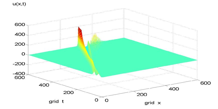
Figure 2: Solitons interaction with parameters of the model:  $\alpha=0.5;$  $\beta=0.125;$  $v_{1}=5.5;$  $v_{2}=7;$  $N=3;$  $M=2$.

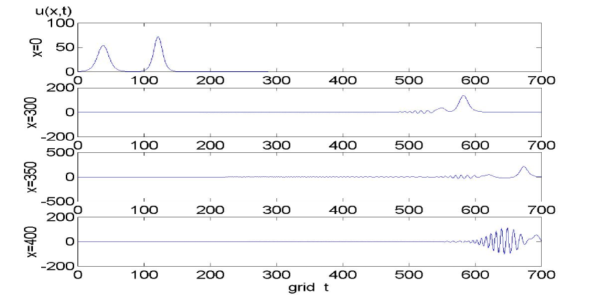
Figure 3: Spatial shears of the solitons interaction with parameters of the model:  $\alpha=0.5;$  $\beta=0.125;$  $v_{1}=5.5;$  $v_{2}=7;$  $N=3;$  $M=2$.

On  Fig.2 is presented an instance of the solitons interaction with the velocities ratio outside of noted above areas:  $m_{1}=0.55$; $m_{2}=0.7$. The interaction occurs inelastically. On  Fig.3 is presented the consequence of shears of the wave before and after the interaction. From figures is seen that approximately only about half on amplitude and length of the quick soliton continues the motion with the previous velocity as the solitary wave. The length of this wave is a half of the length of the slow soliton. The slow soliton absorbed part of the quick soliton energy and transformed in the shock wave with the same scenario of the behaviour, as on  Fig.1.

If consider solitons as a sum of harmonical waves then from presented results follows that exist tunnel zones in neighborhood of multiple magnitudes of the velocities, when harmonic components mutually penetrate. Outside of the tunnel zones more slow wave emerges as potential barrier, through which passes the part of harmonical waves, period which is multiple with respect to length of the barrier. Rest harmonical waves enter in nonlinear interaction with the barrier and create the shock wave. Part of waves, which passed the barrier, creates stable on the form solitary wave, moving with previous velocity. As can be seen from the expression  (2), such wave can be considered as solution of the equation  (1) with proportionally increased coefficients $(\alpha;\beta)$. Consequently, resonance to the nonlinear medium can be SW, which parameters give appropriate balance of the form and velocity.

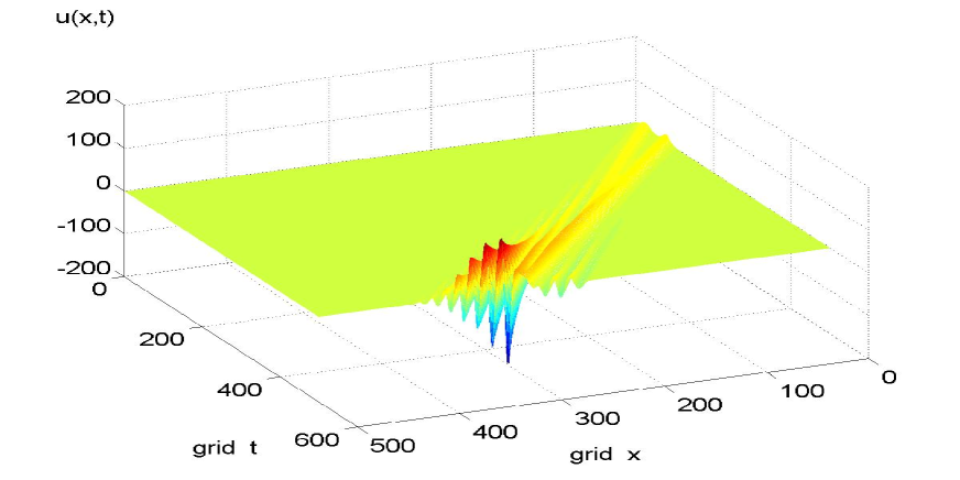
Figure 4: Solitons interaction with parameters of the model:  $\alpha=1;$  $\beta=0.5;$  $v_{1}=6;$  $v_{2}=7;$  $N=2;$  $M=3$.

In the equation  (1) with parameters  (1;0.5),  (1;-3) the nonlinear component has more deep influence. Therefore mutual penetration of the waves with small distortion was observed only in the tunnel zones with $K\geq 2$. On  Fig.4 is presented the solitons interaction of the RLW equation (1;0.5) with parameters of the model:  $N=2$;  $M=3$;  $m_{1}=0.6$;  $m_{2}=0.7$. The interaction runs with formation before front of the slow soliton the third wave, which gradually accumulates the main part of total energy of the solitons and develops in the shock wave, and next in wave like  (4). In this case the transition in the wave like  (4) is realized quicker and so the shock wave excites the series of the fluctuations developing in periodical singularites. The third wave is formed as reflection of the slow wave from running up front of the quick wave. Then reflected wave absorbs quick soliton. Such interaction shows that with increase the influence of a nonlinearity grows the ability of the solitons to save the form. The interaction of the solitons of the RLW equation with parameters (1;-3) occurs similarly and differs the inverse sign of the wave.

Presented in article the model has allowed to see result of influence of the nonlinearity on non-equilibrium interaction of the SW. As a groundwork to influence is used the linear model (7), which is equivalent to superposition of the operators (5) each of SW.

$$\left\{\prod_{n=1}^{N}\left(\frac{\partial}{\partial t}+v_{n}\frac{\partial}{\partial x}\right)^{p_{n}}\right\}u(x,t)=0,$$

where $p_{n}$ are integer values, which regulate the filtering characteristic each of multiplier. For realization of the computing scheme  (10) the auxiliary linear model can be formed for each layer or counting sample on its neighbourhood. The linear model must be unitary to not influence on processes of damping and excitation of fluctuations. With the help of linear model was eliminated ambiguity of nonlinear equation solution by matching on a dynamic of current and previous samples. Model was researched also with discrete analogue of the nonlinearity as $u_{i,j-1}(u_{i,j}-u_{i,j-2})/2\Delta x$. Such model gave the results, similar mentioned above, but it was less stable in contrast with  (10) and amplitude of the shock wave did’t rise up to saturation level.

Possible suppose that transformation of the shock wave in the wave like  (4) occurs under influence of $\gamma u_{x}$ in equation  (1). To value the level of this factor the model, presented on  Fig.1, was researched for $\gamma=-0.25\dots 1.5$. It was determined that ratio of the amplitude of the shock wave saturation to the average magnitude of the solitons amplitudes is valued as about $24-8\gamma$ and though amplitudes of the solitons with reduction $\gamma$ increase the time of the shock wave saturation grows as about $T(\gamma=1)+160\Delta t(1-\gamma)$. These results show that $\gamma$ affects only partly – with the reduction of $\gamma$ decreases ability to saturation. Since a shock wave with high amplitude is’t a solution of the RLW equation with any parameter $\gamma$, that the main factor is a process of self-organization of the shock wave under influence of the factors of amplitude, frontage and velocity, in consequence of which the shock wave shapes up the resonance form that is acceptable from condition of the high derivatives balance. This is confirmed following, when the solitons amplitude was changed by parameter $v_{0}=10\dots 200$ the ratio of the amplitude of the shock wave saturation to average magnitude of the solitons amplitudes was valued as about $8{v_{0}}^{0.3}$ and the time of saturation greatly was’t changed. However, was found ranges where does’t occur the shock wave saturation: $v_{0}=70\dots 80$; 125…150; 180…200. The shock waves with high amplitude are formed in these ranges right after collision, or in cross point of the SW. Whereupon the model lost stability. In addition, the double order was needed for stable linear model in these ranges. The model of the KdV equation behaved similarly.

When $v\gg\gamma$ the spectral parameter in equation  (3) $a\approx\sqrt{1/\alpha}$ and so solitons of the RLW equation are spatially quasicoherent. Hence, the nonequilibrium interaction of the quasicoherent solitons can generates solitary and shock waves, self-excited quick waves-harbingers. The shock wave can reach to be tenfold amplitude in contrast with generating it solitons due to the profile narrowing. In the case of weak nonlinearity possible partial mutual penetration with formation of saving form solitary waves. Strong nonlinearity brings about forming the third wave, which accumulates the main part forming it the solitons. The self-excitation of the quick waves-harbingers can be considered as property of a nonlinear medium spontaneously to generate fluctuations under influence of small perturbations.

The model has reflected conversion of the nonlinear medium from one type of the balance of the amplitude and velocity – two solitons  (3), to the other, in the form of the stable positive wave front, which precedes developing in singularity negative front. Physical sense of such transition possible to make clear considering other characteristic of concrete phenomena, described by equation  (1). For example, the RLW equation (0.5;0.125) describes an ion velocity in Broer - Sluijter’s system of equations of plasma  [5]. Numerical modeling of the dynamic of the ion density at the speed on  Fig.1 using the direct matrix method has shown that when ion velocity takes the form of the shock wave with stable amplitude and appears negative front the amplitude of fluctuations of the ion density sharply increases. The negative velocity possible to consider as effect of the elastic force reaction on quick ions. The rapprochement with the singular point of the velocity brings about forming the fluctuations of the density with high amplitude, spreading in forward and backward directions. Consequently, the singularity corresponds to excited by colliding ions source of the fluctuations of density.

Solitary waves can meet in nature as multiwave systems and as separate formations, depending on this condition runs their interaction. The first type of the interaction well studied by analytical way. Example of the numerical analysis of the second type of the interaction is presented in this article. Results of modeling allow to draw a conclusion that nonlinearity reveals itself ambiguously – in one event exists the mutual penetration, in the other – full or partial interaction with transition in qualitative other resonance state. Partly the interaction of the SW in nonlinear medium possible to describe qualitatively as processes of the multiplying and mutual passing – reflections of their harmonic components taking into account orthogonality of the harmonics and conservations of total energy.

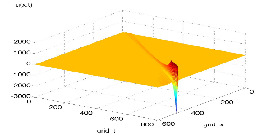
Figure 1: Solitons interaction with parameters of the model:  $\alpha=0.5;$  $\beta=0.125;$  $v_{1}=6.05;$  $v_{2}=6.7;$  $N=3;$  $M=2$.

References

- [1] R. K. Dodd, J. C. Eilbeck, J. D. Gibbon, H. C. Morris. Solitons and Nonlinear Wave Equatation. Academic Press, Inc (London), 1984.
- [2] F. Calogero, A. Degasperis. Spectral transform and solitons. North - Holland Publishing Company, 1982
- [3] M. Q. Tran. Physica Scrita, 20, 317-327 (1979).
- [4] S. L. Marple, Jr. Digital Specral Analysis with applications. Prentice-Hall, Inc. Englewood Cliffs, New Jersey 07632, 1987.
- [5] L. F.J. Broer, F. W. Sluijter. Phys. Fluids, 20, 1458 (1977).